Table of Contents
| DATA ANALYTICS REFERENCE DOCUMENT |
|
|---|---|
| Document Title: | 52465 - Programming for Data Analytics module summary |
| Document No.: | 1540154135 |
| Author(s): | |
| Contributor(s): | Rita Raher, Gerhard van der Linde, Gearoid O'Gcrannaoil |
REVISION HISTORY
| Revision | Details of Modification(s) | Reason for modification | Date | By |
|---|---|---|---|---|
| 0 | Draft release | Create a printable reference documented summary of module highlights | 2018/10/21 20:35 | Gearoid O'Gcrannaoil |
52465 - Programming for Data Analysis
Learning outcomes
On completion of this module1) the learner will/should be able to:
- Perform exploratory analysis on data.
- Programmatically create plots and other visual outputs from data.
- Design computer algorithms to solve numerical problems.
- Create software that incorporates and utilises standard numerical libraries.
- Employ appropriate data structures when programming for data-intensive applications.
- Model real-world, data-intensive problems as computing problems.
Indicative syllabus
The following is a list of topics that will likely be covered in this module. Note that the topics might not be presented in this order and might not be explicitly referenced in course materials.
Data
Two-dimensional arrays, matrices, data frames, time series data structures, dictionaries, sets, vectors, slicing, indexing
Programming
Reshaping data structures, unzipping arrays, slicing, calculating descriptive statistics.
Analytics
Exploratory data analysis, scatterplots, histograms, boxplots, principal component analysis.
Python review

- A review of how to get set up with a repository for starting a new software project.
- A review of if statements in Python.
- A review of while loops in Python.
- A review of for loops in Python.
- A review of functions in Python.
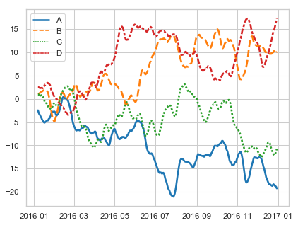
Plotting basics (matplotlib)

This week we will look at the pyplot plotting library for Python.
Browser workflows (jupyter)

This week we will look at the jupyter package for creating visual workflows to tell a data analytics story.
- Starting jupyter
- Renaming notebooks
- Cells in jupyter
- Jupyter keyboard shortcuts
- Code and markdown cells in jupyter
- Jupyter kernel
- Plotting in jupyter
- Jupyter lab
- A gallery of interesting Jupyter Notebooks4)
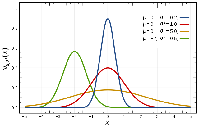
Generating random data (numpy)

This week we will look at the numpy.random package for generating random data in Python.
- An introduction to the numpy.random package.5)
- Getting started with a numpy.random notebook.
- The numpy.random documentation.
- About the rand function in the numpy.random package.
- Seeds in the numpy.random package.10)

 An example of a random “seed“
Exploring data sets (pandas)
- Introduction to pandas
- Introduction to pandas notebook11)
- Reading CSV files in pandas
- Using loc and iloc
- Boolean selects
- Summarising datasets with pandas and seaborn
- Pandas and iris dataset notebook (right click and 'save as')
Highligts from the series
Use pandas to read as csv file into a dataframe and run some basic analytics on it.
- pandas_samples.py
import pandas as pd
df = pd.read_csv("https://raw.githubusercontent.com/uiuc-cse/data-fa14/gh-pages/data/iris.csv")

# show the data type in the dataframe and the names of the columns imported if any
df.dtypes
#show the headings with data
df.head()
# a list of columns
df.columns
# a list of statistics per column
df.describe()
# the mean or median only
df.mean()
df.median()
and show it all in graphs using Seabborn and Pandas
- seaborn_samples.py
import seaborn as sns
import matplotlib.pyplot as pl
sns.pairplot(df, hue='species')
pl.show()
Machine learning (sklearn)
![]()
This week we will look at the sklearn package for machine learning in Python.
- Intro to sklearn. Machine learning in Python - a very Powerful package12)
- Build up a case for a machine learning - visualise the data in a plot before deciding to use K-nearest neighbours. We look at how to split a data set into inputs and outputs for supervised learning.
- How to train a knn classifier in sklearn.
# classifier - takes 5 nearest neighbours
knn = nei.KNeighborsClassifier(n_neighbors=5)

# fit
knn.fit (inputs, outputs)
- How to make predictions from a trained classifier.
knn.predict([[5.1, 3.5, 1.4, 0.2]])
- How to test a classifier. Even on the data values you trained the classifiers, if might not get them correct.
# To Evaluate, you can check and compare to the dataframe using:
knn.predict(inputs) == outputs

# converts all the trues to 1s and false to 0 and adds them
(knn.predict(inputs) == outputs).sum()

#Split arrays or matrices into random train and test subsets

import sklearn.model_selection as mod

inputs_train, inputs_test, outputs_train, outputs_test = mod.train_test_split(inputs, outputs, test_size=0.33)
References: http://scikit-learn.org/
Tutorials http://scikit-learn.org/stable/tutorial/basic/tutorial.html
Other Machine Learning frameworks https://www.tensorflow.org/
Exploring time series (yet more pandas)
- time-series.py
import pandas as pd
df = pd.read_csv("http://cli.met.ie/cli/climate_data/webdata/hly4935.csv", skiprows=23, low_memory=False, nrows=1000)
# Change the date column to a Pythonic datetime.
df['datetime'] = pd.to_datetime(df['date'])
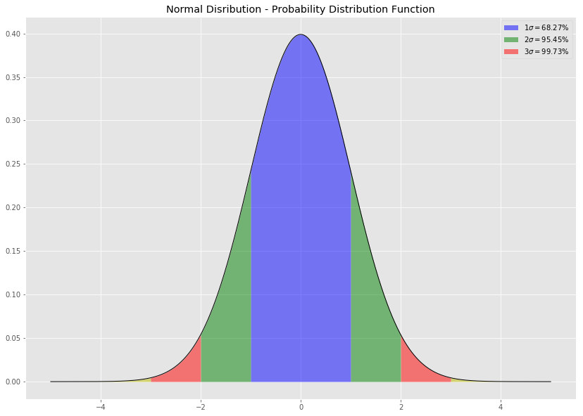
Statistical bias (numpy.random)
Bias
A statistic is biased if, in the long run, it consistently over or underestimates the parameter it is estimating. More technically it is biased if its expected value is not equal to the parameter. A stop watch that is a little bit fast gives biased estimates of elapsed time. Bias in this sense is different from the notion of a biased sample. A statistic is positively biased if it tends to overestimate the parameter; a statistic is negatively biased if it tends to underestimate the parameter. An unbiased statistic is not necessarily an accurate statistic. If a statistic is sometimes much too high and sometimes much too low, it can still be unbiased. It would be very imprecise, however. A slightly biased statistic that systematically results in very small overestimates of a parameter could be quite efficient. 13)
Databases(sqlite)

Summary of the essentials
- sqlite.py
import sqlite3  # load the SQLite library
conn = sqlite3.connect('data/example.db') # open a local database file
c = conn.cursor() # create a cursor c

#read three csv files in
person = pd.read_csv("https://github.com/ianmcloughlin/datasets/raw/master/cars-db/person.csv", index_col=0)
car = pd.read_csv("https://github.com/ianmcloughlin/datasets/raw/master/cars-db/car.csv", index_col=0)
county = pd.read_csv("https://github.com/ianmcloughlin/datasets/raw/master/cars-db/county.csv", index_col=0)

#convert and save csv files to the database
county.to_sql("county", conn)
person.to_sql("person", conn)
car.to_sql("car", conn)

# run a query to show all the tables created above
c.execute("SELECT name FROM sqlite_master WHERE type='table'")
c.fetchall()

# run a query with a joinbetween two tables
c.execute("""
    SELECT p.Name, c.Registration, p.Address
    FROM person as p JOIN car as c ON p.ID = c.OwnerId
""")
c.fetchall()

# run a query with a join between three tables
c.execute("""
    SELECT p.Name, c.Registration, p.Address
    FROM person as p
         JOIN car as c ON p.ID = c.OwnerId
         JOIN county as t ON t.Name = p.Address
    WHERE c.Registration NOT LIKE '%-' + t.Registration + '-%'
""")
c.fetchall()

# close the connection
conn.close()
IPython

closely linKed to jupyter. Ipython runs on the command line. ipython comes by default with the anaconda distribution. use the up arrows to navigate previous commands. It works as a python interpreter. You can import the usual packages.
Run ipython in the command line
import numpy as np
np.arange(0.0, 10.0, 0.1)
python: python statements
import numpy as np
np.linspace(0.0, 10.0, 100)

import matplotlib.pyplot as plt

plt.plot(np.linspace(0.0, 10.0, 100)
plt.show()
and a new window shows up! code the window to get a new prompt from ipython
It remembers all the variables you have created. type “exit” to get out of ipython
ipython: %paste
paste magin command
https://ipython.readthedocs.io/en/stable/interactive/magics.html
for i in range(10):
	print(i, i**2)
Paste in python code from python tutorials and ipython will run it https://docs.python.org/3/tutorial/controlflow.html
>>> for n in range(2, 10):
...     for x in range(2, n):
...         if n % x == 0:
...             print(n, 'equals', x, '*', n//x)
...             break
...     else:
...         # loop fell through without finding a factor
...         print(n, 'is a prime number’)
Best practice is to copy the code and then type %paste into the command line and this will run the script %paste
ipython: %timeit
%timeit [i**2 for i in range(100)]
30.4 µs ± 668 ns per loop (mean ± std. dev. of 7 runs, 10000 loops each)
%timeit np.arange(100)**2
1.17 µs ± 13.1 ns per loop (mean ± std. dev. of 7 runs, 1000000 loops each)
ipython: %run
- %pwd - present working directory
- %cd - change directory
- %cd Desktop/
- %ls - lists files
- %cls - clears everything
- %run filename.py
- %reset - removes variables