modules:52954
Table of Contents
| DATA ANALYTICS REFERENCE DOCUMENT |
|
|---|---|
| Document Title: | Document Title |
| Document No.: | 1569147909 |
| Author(s): | Gerhard van der Linde, Rita Raher |
| Contributor(s): | |
REVISION HISTORY
| Revision | Details of Modification(s) | Reason for modification | Date | By |
|---|---|---|---|---|
| 0 | Draft release | Document description here | 2019/09/22 10:25 | Gerhard van der Linde |
52954 - Machine Learning and Statistics
Week 1 - Python Review
Python review
Python Setup
What is a typical Python development environment set up?
Revising Collatz
The Collatz conjecture: how do you write a small Python program?
Create a new git repository
How do you create a new git repository for a project?
Create a Jupyter notebook
How do you create a new Jupyter notebook synced with GitHub?
The Top Programming Languages 2019 by Stephen Cass
https://spectrum.ieee.org/computing/software/the-top-programming-languages-2019
Article from the IEEE about their analysis of the most popular programming languages in 2019.
Python fundamentals
Jupyter notebook refreshing the fundamentals of the Python language.
Anaconda
https://www.anaconda.com/distribution/
Down the Anaconda Python distribution.
Python.org
Official Python website.
Dive into Python 3
http://diveintopython3.problemsolving.io/
Dive into Python 3 - a tutorial on Python 3 for programmers.
Week 2 - Stochasticism
Stochasticism
stochastic
ADJECTIVE
technical
having a random probability distribution or pattern that may be analysed statistically but may not be predicted precisely.
synonyms: unsystematic · arbitrary · unmethodical · haphazard · unarranged · unplanned · undirected · casual · indiscriminate · non-specific · stray · erratic · chance · accidental · hit-and-miss · serendipitous · fortuitous · contingent · adventitious · non-linear · entropic · fractal · aleatory
Reference Material
Notebook: coin flipping
https://nbviewer.jupyter.org/github/ianmcloughlin/jupyter-teaching-notebooks/blob/master/coin-flip.ipynb https://nbviewer.jupyter.org/github/G00364778/52954_Machine_Learning_and_Statistics/blob/master/coin_flip.ipynb
A notebook about the binomial distribution.
Website: Stat Trek - Binomial Distribution
https://stattrek.com/probability-distributions/binomial.aspx
Stat Trek's page on the binomial distribution.
Website: NIST Engineering Statistics Handbook - Binomial Distribution
https://www.itl.nist.gov/div898/handbook/eda/section3/eda366i.htm
Binomial Distribution page from the (USA) National Institute of Standards and Technology.
Video: Creating Jupyter notebooks
https://web.microsoftstream.com/video/8e965392-ccc2-4faa-a755-8d86de6a91d6
How to run Jupyter, create a notebook, and sync it to GitHub.
Video: Computing and coin flipping
https://web.microsoftstream.com/video/930f0c96-3fbd-4b9a-bcb0-51af0e522da4
How are coin flipping and computing related?
Video: Coin flipping in Python
https://web.microsoftstream.com/video/2cd606c0-3269-4a2d-975d-f089514b8bfc
Using Python to simulate coin flipping.
Summary
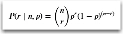
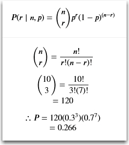
So applying the math to the formula with 10 coin flips resulting in three heads, the probability P is:
Week 3 - Mathematical models
Reference Material
Mathematical models
Variables in pyplot
import matplotlib.pyplot as plt
import numpy as np

x = np.linspace(0,100,11)
y = np.exp(x)

plt.plot(x,y,'r.')
Simple Linear regression
The essentials from linear regression is summarised in the python code below discussing the spring length(d) for the various weights(w).
Newton's method in Python
https://en.wikipedia.org/wiki/Newton%27s_method
# Adapted from: https://tour.golang.org/flowcontrol/8

def sqrt(x):
  # Initial guess.
  z = 1.0
  # Keep getting a better estimate for the square root
  # of x, until you are within two decimal places.
  while abs(z*z - x) >= 0.0001:
    # Get a better approximation for the square root.
    z -= (z*z - x) / (2*z)
  # Return z.
  return z

# Calculate the square root of 8.
z = sqrt(63.0)
# Print z.
print(z)
# Print the square of the square of z.
print(z*z)
Week 4 - Regression
References
https://realpython.com/linear-regression-in-python/
Notes from blog post:
- The dependent features are called the dependent variables, outputs, or responses.
- The independent features are called the independent variables, inputs, or predictors.
Practical Linear Regression
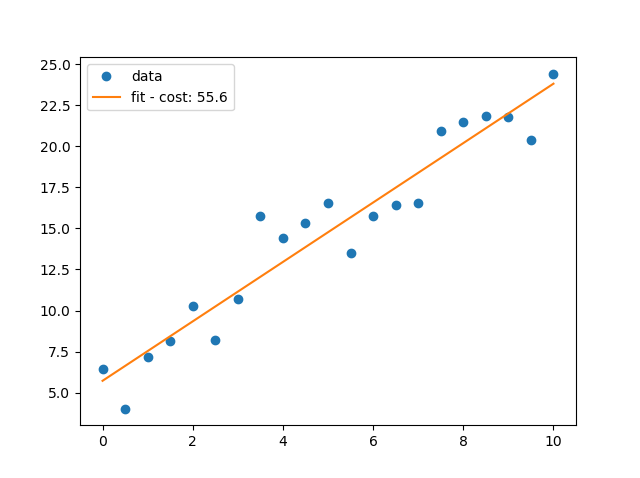
# import the required libraries
import matplotlib.pyplot as pl
import numpy as np

x=np.arange(0.0,10.1,0.5)
y=2*x+5+np.random.normal(0,np.mean(x)/3,len(x))
m,c = np.polyfit(x,y,1)

cost=y-(m*x+c)
cost='fit - cost: {:3.1f}'.format(np.sum(cost**2))

pl.ioff()
pl.plot(x,y,'o',label='data')
pl.plot(x, m * x + c, '-', label=cost)
pl.legend()
pl.show()
Multi-linear regression using sklearn
<m 18> petalwidth = t (sepallength) + u (sepalwidth) + v (petallength) + c </m>
Using sklearn
- multi_sk.py
# Import linear_model from sklearn.
import sklearn.linear_model as lm

# Create a linear regression model instance.
m = lm.LinearRegression()

# Let's use pandas to read a csv file and organise our data.
import pandas as pd

# Read the iris csv from online.
df = pd.read_csv('https://datahub.io/machine-learning/iris/r/iris.csv')

# Let's pretend we want to do linear regression on these variables to predict petal width.
x = df[['sepallength', 'sepalwidth', 'petallength']]

# Here's petal width.
y = df['petalwidth']

# Ask our model to fit the data.
m.fit(x, y)

# Here's our intercept.
print('   intercept: ',m.intercept_)

# Here's our coefficients, in order.
print('coefficients: ',m.coef_)

# See how good our fit is.
print('       score: ',m.score(x, y))
   intercept:  -0.248723586024455
coefficients:  [-0.21027133  0.22877721  0.52608818]
       score:  0.9380481344518986
Using statsmodels
- multi_stats.py
# Using statsmodels.
import statsmodels.api as sm

# Tell statmodels to include an intercept.
xwithc = sm.add_constant(x)

# Create a model.
msm = sm.OLS(y, xwithc)
# Fit the data.
rsm = msm.fit()
# Print a summary.
print(rsm.summary())
                            OLS Regression Results
==============================================================================
Dep. Variable:             petalwidth   R-squared:                       0.938
Model:                            OLS   Adj. R-squared:                  0.937
Method:                 Least Squares   F-statistic:                     736.9
Date:                Sun, 06 Oct 2019   Prob (F-statistic):           6.20e-88
Time:                        16:54:18   Log-Likelihood:                 36.809
No. Observations:                 150   AIC:                            -65.62
Df Residuals:                     146   BIC:                            -53.57
Df Model:                           3
Covariance Type:            nonrobust
===============================================================================
                  coef    std err          t      P>|t|      [0.025      0.975]
-------------------------------------------------------------------------------
const          -0.2487      0.178     -1.396      0.165      -0.601       0.103
sepallength    -0.2103      0.048     -4.426      0.000      -0.304      -0.116
sepalwidth      0.2288      0.049      4.669      0.000       0.132       0.326
petallength     0.5261      0.024     21.536      0.000       0.478       0.574
==============================================================================
Omnibus:                        5.603   Durbin-Watson:                   1.577
Prob(Omnibus):                  0.061   Jarque-Bera (JB):                6.817
Skew:                           0.222   Prob(JB):                       0.0331
Kurtosis:                       3.945   Cond. No.                         90.0
==============================================================================

Warnings:
[1] Standard Errors assume that the covariance matrix of the errors is correctly specified.
Week 5 - T-tests
Independent t-test using SPSS Statistics
Introduction
The independent-samples t-test (or independent t-test, for short) compares the means between two unrelated groups on the same continuous, dependent variable. For example, you could use an independent t-test to understand whether first year graduate salaries differed based on gender (i.e., your dependent variable would be “first year graduate salaries” and your independent variable would be “gender”, which has two groups: “male” and “female”). Alternately, you could use an independent t-test to understand whether there is a difference in test anxiety based on educational level (i.e., your dependent variable would be “test anxiety” and your independent variable would be “educational level”, which has two groups: “undergraduates” and “postgraduates”).
This “quick start” guide shows you how to carry out an independent t-test using SPSS Statistics, as well as interpret and report the results from this test. However, before we introduce you to this procedure, you need to understand the different assumptions that your data must meet in order for an independent t-test to give you a valid result. We discuss these assumptions next.
Assumptions
When you choose to analyse your data using an independent t-test, part of the process involves checking to make sure that the data you want to analyse can actually be analysed using an independent t-test. You need to do this because it is only appropriate to use an independent t-test if your data “passes” six assumptions that are required for an independent t-test to give you a valid result. In practice, checking for these six assumptions just adds a little bit more time to your analysis, requiring you to click a few more buttons in SPSS Statistics when performing your analysis, as well as think a little bit more about your data, but it is not a difficult task.
Before we introduce you to these six assumptions, do not be surprised if, when analysing your own data using SPSS Statistics, one or more of these assumptions is violated (i.e., is not met). This is not uncommon when working with real-world data rather than textbook examples, which often only show you how to carry out an independent t-test when everything goes well! However, don't worry. Even when your data fails certain assumptions, there is often a solution to overcome this. First, let's take a look at these six assumptions:
- Assumption #1: Your dependent variable should be measured on a continuous scale (i.e., it is measured at the interval or ratio level). Examples of variables that meet this criterion include revision time (measured in hours), intelligence (measured using IQ score), exam performance (measured from 0 to 100), weight (measured in kg), and so forth. You can learn more about continuous variables in our article: Types of Variable.
- Assumption #2: Your independent variable should consist of two categorical, independent groups. Example independent variables that meet this criterion include gender (2 groups: male or female), employment status (2 groups: employed or unemployed), smoker (2 groups: yes or no), and so forth.
- Assumption #3: You should have independence of observations, which means that there is no relationship between the observations in each group or between the groups themselves. For example, there must be different participants in each group with no participant being in more than one group. This is more of a study design issue than something you can test for, but it is an important assumption of the independent t-test. If your study fails this assumption, you will need to use another statistical test instead of the independent t-test (e.g., a paired-samples t-test). If you are unsure whether your study meets this assumption, you can use our Statistical Test Selector, which is part of our enhanced content.
- Assumption #4: There should be no significant outliers. Outliers are simply single data points within your data that do not follow the usual pattern (e.g., in a study of 100 students' IQ scores, where the mean score was 108 with only a small variation between students, one student had a score of 156, which is very unusual, and may even put her in the top 1% of IQ scores globally). The problem with outliers is that they can have a negative effect on the independent t-test, reducing the validity of your results. Fortunately, when using SPSS Statistics to run an independent t-test on your data, you can easily detect possible outliers. In our enhanced independent t-test guide, we: (a) show you how to detect outliers using SPSS Statistics; and (b) discuss some of the options you have in order to deal with outliers. You can learn more about our enhanced independent t-test guide here.
- Assumption #5: Your dependent variable should be approximately normally distributed for each group of the independent variable. We talk about the independent t-test only requiring approximately normal data because it is quite “robust” to violations of normality, meaning that this assumption can be a little violated and still provide valid results. You can test for normality using the Shapiro-Wilk test of normality, which is easily tested for using SPSS Statistics. In addition to showing you how to do this in our enhanced independent t-test guide, we also explain what you can do if your data fails this assumption (i.e., if it fails it more than a little bit). Again, you can learn more here.
- Assumption #6: There needs to be homogeneity of variances. You can test this assumption in SPSS Statistics using Levene’s test for homogeneity of variances. In our enhanced independent t-test guide, we (a) show you how to perform Levene’s test for homogeneity of variances in SPSS Statistics, (b) explain some of the things you will need to consider when interpreting your data, and © present possible ways to continue with your analysis if your data fails to meet this assumption (learn more here).
You can check assumptions #4, #5 and #6 using SPSS Statistics. Before doing this, you should make sure that your data meets assumptions #1, #2 and #3, although you don't need SPSS Statistics to do this. When moving on to assumptions #4, #5 and #6, we suggest testing them in this order because it represents an order where, if a violation to the assumption is not correctable, you will no longer be able to use an independent t-test (although you may be able to run another statistical test on your data instead). Just remember that if you do not run the statistical tests on these assumptions correctly, the results you get when running an independent t-test might not be valid. This is why we dedicate a number of sections of our enhanced independent t-test guide to help you get this right. You can find out about our enhanced independent t-test guide here, or more generally, our enhanced content as a whole here.
In the section, Test Procedure in SPSS Statistics, we illustrate the SPSS Statistics procedure required to perform an independent t-test assuming that no assumptions have been violated. First, we set out the example we use to explain the independent t-test procedure in SPSS Statistics.
Example
The concentration of cholesterol (a type of fat) in the blood is associated with the risk of developing heart disease, such that higher concentrations of cholesterol indicate a higher level of risk, and lower concentrations indicate a lower level of risk. If you lower the concentration of cholesterol in the blood, your risk of developing heart disease can be reduced. Being overweight and/or physically inactive increases the concentration of cholesterol in your blood. Both exercise and weight loss can reduce cholesterol concentration. However, it is not known whether exercise or weight loss is best for lowering cholesterol concentration. Therefore, a researcher decided to investigate whether an exercise or weight loss intervention is more effective in lowering cholesterol levels. To this end, the researcher recruited a random sample of inactive males that were classified as overweight. This sample was then randomly split into two groups: Group 1 underwent a calorie-controlled diet and Group 2 undertook the exercise-training programme. In order to determine which treatment programme was more effective, the mean cholesterol concentrations were compared between the two groups at the end of the treatment programmes.
Independent T-Test using Python
With the advent of computers, we can now calculate your t-value, and then instead of looking up a challenge based on alpha = 5%, we can instead calculate what alpha is for your exact t-value that you calculated. This is the p-value. If p < alpha = 0.05, you have a statistically significant difference.1)
Jupyter notebook exported using Pandoc2)
import scipy.stats as ss
ss.ttest_ind
<function scipy.stats.stats.ttest_ind(a, b, axis=0, equal_var=True, nan_policy='propagate')>
import numpy as np
m = np.random.normal(1.7, 0.1, 30) # create a distribution for males
i = np.random.normal(1.7, 0.1, 30) # create a second distribution for males for comparison
f = np.random.normal(1.6, 0.1, 30) # and one for females
m
array([1.65608233, 1.53733214, 1.70894662, 1.63391829, 1.79362808,
       1.80130406, 1.68387788, 1.78518434, 1.7137346 , 1.73436257,
       1.57993658, 1.79873049, 1.85459491, 1.62009294, 1.57099436,
       1.70454494, 1.58636796, 1.76735163, 1.57995404, 1.79756806,
       1.78004978, 1.87028346, 1.55481802, 1.52903448, 1.73452971,
       1.79966479, 1.7315535 , 1.65528311, 1.69771424, 1.66517462])
f
array([1.51043915, 1.47669289, 1.6932561 , 1.43280066, 1.61460339,
       1.81777216, 1.68714345, 1.54090906, 1.59801562, 1.68750582,
       1.58823061, 1.81329238, 1.50000238, 1.59306356, 1.65096888,
       1.51298434, 1.38841657, 1.52372802, 1.64747762, 1.50317819,
       1.66220508, 1.76229033, 1.4329828 , 1.7723186 , 1.66407174,
       1.57042659, 1.64804087, 1.55661205, 1.71034986, 1.59118956])
i
array([1.7909649 , 1.53540857, 1.60156219, 1.79307352, 1.81230742,
       1.71791994, 1.6865362 , 1.73692561, 1.7631472 , 1.66366704,
       1.67118224, 1.78938662, 1.48725615, 1.5188362 , 1.61369048,
       1.4665699 , 1.69378468, 1.61759276, 1.817376  , 1.76087075,
       1.6173938 , 1.65284768, 1.7989501 , 1.77414378, 1.72655364,
       1.73790678, 1.72574204, 1.67446458, 1.81852192, 1.77273642])
ss.ttest_ind(m, f)
Ttest_indResult(statistic=3.4195352674685178, pvalue=0.001154202030644732)
ss.ttest_ind(m, i)
Ttest_indResult(statistic=0.11658982658666799, pvalue=0.9075878717154473)
import statsmodels.stats.weightstats as ws
ws.ttest_ind(m, f)
(3.4195352674685187, 0.0011542020306447302, 58.0)
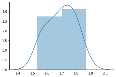
import seaborn as sns
sns.distplot(m)
<matplotlib.axes._subplots.AxesSubplot at 0x2cd36f5f908>
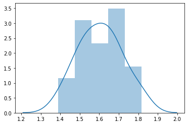
sns.distplot(f)
<matplotlib.axes._subplots.AxesSubplot at 0x2cd3826ca58>
import pandas as pd
df = pd.DataFrame({'male': m, 'female': f})
df
        male    female
0   1.656082  1.510439
1   1.537332  1.476693
2   1.708947  1.693256
3   1.633918  1.432801
   ...
27  1.655283  1.556612
28  1.697714  1.710350
29  1.665175  1.591190
ss.ttest_ind(df['male'], df['female'])
Ttest_indResult(statistic=3.4195352674685178, pvalue=0.001154202030644732)
gender = ['male'] * 30 + ['female'] * 30
height = np.concatenate([m, f])
df = pd.DataFrame({'gender': gender, 'height': height})
df
    gender    height
0     male  1.656082
1     male  1.537332
2     male  1.708947
3     male  1.633918
  ...
27    male  1.655283
28    male  1.697714
29    male  1.665175
30  female  1.510439
31  female  1.476693
  ...
57  female  1.556612
58  female  1.710350
59  female  1.591190
df[df['gender'] == 'male']['height']
0     1.656082
1     1.537332
2     1.708947
3     1.633918
  ...
27    1.655283
28    1.697714
29    1.665175
Name: height, dtype: float64
df[df['gender'] == 'female']['height']
30    1.510439
31    1.476693
32    1.693256
  ...
56    1.648041
57    1.556612
58    1.710350
59    1.591190
Name: height, dtype: float64
ws.ttest_ind(df[df['gender'] == 'male']['height'], df[df['gender'] == 'female']['height'])
(3.4195352674685187, 0.0011542020306447302, 58.0)
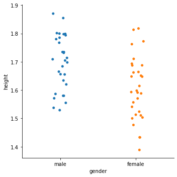
sns.catplot(x='gender', y='height', jitter=True, data=df)
<seaborn.axisgrid.FacetGrid at 0x2cd382e2240>
Week 6 - ANOVA
-
- Ian's notebook on ANOVA, with lots about t-tests and hypothesis testing in general.
-
- Blog post on using statsmodels to perform an ANOVA.
-
- There are many variations of ANOVA with similar sounding names. This blog post summarises a few.
-
- Interesting Stack Exchange post on the differences between ANOVA, ANCOVA and regression.
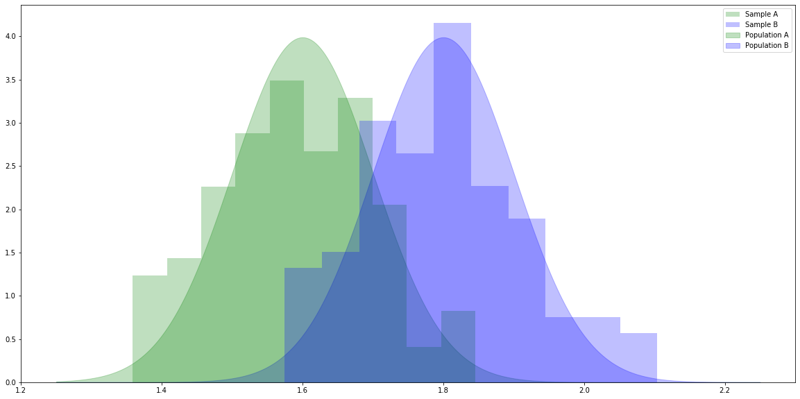
Analysis of variance (ANOVA)
# For generating random variables.
import numpy as np
# For handling data.
import pandas as pd
# For plotting.
import matplotlib.pyplot as plt
# For t-tests and ANOVA.
import scipy.stats as stats

# Make the plots bigger.
plt.rcParams['figure.figsize'] = (20.0, 10.0)

# Set parameters for two populations.
popA = {'m': 1.6, 's': 0.1}
popB = {'m': 1.8, 's': 0.1}

# Create two samples, one from each population.
sampA = np.random.normal(popA['m'], popA['s'], 100)
sampB = np.random.normal(popB['m'], popB['s'], 100)

# x values for plotting.
x = np.linspace(1.25, 2.25, 1000)

# The probability density functions (PDFs) for the two populations.
pdfA = stats.norm.pdf(x, popA['m'], popA['s'])
pdfB = stats.norm.pdf(x, popB['m'], popB['s'])

# Plot the population PDFs as shaded regions.
plt.fill_between(x, pdfA, color='g', alpha=0.25, label="Population A")
plt.fill_between(x, pdfB, color='b', alpha=0.25, label="Population B")

# Plot histograms of the two samples.
plt.hist(sampA, density=True, color='g', alpha=0.25, label="Sample A")
plt.hist(sampB, density=True, color='b', alpha=0.25, label="Sample B")

# Display a legend.
plt.legend()
plt.show()
# Calculate the independent samples t-statistic for the samples.
# We also get the probability of seeing samples at least as different as these given the population means are equal.
stats.ttest_ind(sampA, sampB)
Ttest_indResult(statistic=-13.533089946578349, pvalue=5.6476147781328965e-30)
T-tests with Iris
df = pd.read_csv('https://raw.githubusercontent.com/uiuc-cse/data-fa14/gh-pages/data/iris.csv')
#df

s = df[df['species'] == 'setosa']
r = df[df['species'] == 'versicolor']
a = df[df['species'] == 'virginica']

print(stats.ttest_ind(s['petal_length'], r['petal_length']))
print(stats.ttest_ind(s['petal_length'], a['petal_length']))
print(stats.ttest_ind(r['petal_length'], a['petal_length']))

print(stats.ttest_ind(s['petal_width'], r['petal_width']))
print(stats.ttest_ind(s['petal_width'], a['petal_width']))
print(stats.ttest_ind(r['petal_width'], a['petal_width']))

print(stats.ttest_ind(s['sepal_length'], r['sepal_length']))
print(stats.ttest_ind(s['sepal_length'], a['sepal_length']))
print(stats.ttest_ind(r['sepal_length'], a['sepal_length']))

print(stats.ttest_ind(s['sepal_width'], r['sepal_width']))
print(stats.ttest_ind(s['sepal_width'], a['sepal_width']))
print(stats.ttest_ind(r['sepal_width'], a['sepal_width']))
Ttest_indResult(statistic=-39.46866259397272, pvalue=5.717463758170621e-62)
Ttest_indResult(statistic=-49.965703359355636, pvalue=1.5641224158883576e-71)
Ttest_indResult(statistic=-12.603779441384985, pvalue=3.1788195478061495e-22)
Ttest_indResult(statistic=-34.01237858829048, pvalue=4.589080615710866e-56)
Ttest_indResult(statistic=-42.738229672411165, pvalue=3.582719502316063e-65)
Ttest_indResult(statistic=-14.625367047410148, pvalue=2.2304090710248333e-26)
Ttest_indResult(statistic=-10.52098626754911, pvalue=8.985235037487077e-18)
Ttest_indResult(statistic=-15.386195820079404, pvalue=6.892546060674059e-28)
Ttest_indResult(statistic=-5.629165259719801, pvalue=1.7248563024547942e-07)
Ttest_indResult(statistic=9.282772555558111, pvalue=4.362239016010214e-15)
Ttest_indResult(statistic=6.289384996672061, pvalue=8.916634067006443e-09)
Ttest_indResult(statistic=-3.2057607502218186, pvalue=0.0018191004238894803)
Problems with t-tests
Some links about the main problem we encounter with t-testing.
Website: Multiple t tests and Type I error
http://grants.hhp.coe.uh.edu/doconnor/PEP6305/Multiple%20t%20tests.htm//
Webpage about multiple t tests and Type I errors.
—-
Wikipedia: Multiple Comparisons Problem
https://en.wikipedia.org/wiki/Multiple_comparisons_problem//
Wikipedia page about the multiple comparisons problem.
Multiple t tests and Type I error
- As a simple example, you know that there is a 0.50 probability of obtaining “heads” in a coin flip. If I flip the coin four times, what is the probability of obtaining a heads one or more times across all four flips?
- For two coin flips, the probability of not obtaining at least one heads (i.e., getting tails both times) is $0.50 × 0.50 = 0.25$.
- The probability of one or more heads in two coin flips is $1 – 0.25 = 0.75$. Three-fourths of “two coin flips” will have at least one heads.
- So, if I flip the coin four times, the probability of one or more heads is $1 – (0.50 × 0.50 × 0.50 × 0.50) = 1 – (0.50)4 = 1 – 0.625 = 0.9375$; you will get one or more heads in about $94%$ of sets of “four coin flips”. ***
- Similarly, for a statistical test (such as a t test) with $α= 0.05$, if the null hypothesis is true then the probability of not obtaining a significant result is $1 – 0.05 = 0.95$.
- Multiply $0.95$ by the number of tests to calculate the probability of not obtaining one or more significant results across all tests. For two tests, the probability of not obtaining one or more significant results is $0.95 × 0.95 = 0.9025$.
- Subtract that result from $1.00$ to calculate the probability of making at least one type I error with multiple tests: $1 – 0.9025 = 0.0975$.
- Example: You are comparing 4 groups (A, B, C, D). You compare these six pairs ($α= 0.05$ for each): AH vs B, B vs C, C vs D, A vs C, A vs D, and B vs D.
- Using the convenient formula, the probability of not obtaining a significant result is $1 – (1 – 0.05)6 = 0.265$, which means your chances of incorrectly rejecting the null hypothesis (a type I error) is about 1 in 4 instead of 1 in 20!!
- ANOVA compares all means simultaneously and maintains the type I error probability at the designated level.
plt.hist(r['sepal_length'], label='Versicolor Sepal Length')
plt.hist(a['sepal_length'], label='Virginica Sepal Length')

plt.legend()

plt.show()

1- ((0.95)**12)
0.45963991233736334
stats.f_oneway(s['petal_length'], r['petal_length'], a['petal_length'])
F_onewayResult(statistic=1179.0343277002194, pvalue=3.0519758018278374e-91)
plt.hist(s['petal_length'], label='Setosa Petal Length')
plt.hist(r['petal_length'], label='Versicolor Petal Length')
plt.hist(a['petal_length'], label='Virginica Petal Length')

plt.legend()

plt.show()

About t-tests
When performing an independent sample t-test we assume that there is a given difference between the means of two populations, usually a difference of zero.
We then look at the samples to investigate how different they are, calculating their t-statistic.
We then ask, given the hypothesised difference (usually zero) what was the probability of seeing a t-statistic at least this extreme.
If it's too extreme (say, less that 5% chance of seeing it) then we say our hypothesis about the difference must be wrong.
Errors
Of course, we might, by random chance, see a t-statistic that extreme.
We might reject the hypothesis incorrectly - the populations might have the hypothesised difference and the samples just randomly happened to be as different as they are.
We call that a Type I error.
We also might not reject the hypothesis when it's not true - that's a Type II error.

Calculating the t-statistic
From the WikiPedia pages for Student's t-test and Variance.
Note that we are using the calculations for two samples, with equal variances, and possibly different sample sizes.
$$ {\displaystyle t={\frac bar_x_{1}-{\bar {X}}_{2}}{s_{p}\cdot {\sqrt frac_1_n_1}+{\frac {1}{n_{2}}}}}}}} $$
$$ {\displaystyle s_{p}={\sqrt {\frac {\left(n_{1}-1\right)s_{X_{1}}^{2}+\left(n_{2}-1\right)s_{X_{2}}^{2}}{n_{1}+n_{2}-2}}}} $$
$$ {\displaystyle s^{2}={\frac {1}{n-1}}\sum _{i=1}^{n}\left(Y_{i}-{\overline {Y}}\right)^{2}} $$

Note: The latex code is hidden above the image, view in edit mode.
# Count the samples.
nA = float(len(sampA))
nB = float(len(sampB))

# Calculate the means.
mA = sampA.sum() / nA
mB = sampB.sum() / nB

# Sample variances.
varA = ((sampA - mA)**2).sum() / (nA - 1.0)
varB = ((sampB - mB)**2).sum() / (nB - 1.0)

# Pooled standard deviation.
sp = np.sqrt(((nA - 1.0) * varA + (nB - 1.0) * varB) / (nA + nB - 2.0))

# t-statistic
t = (mA - mB) / (sp * np.sqrt((1.0 / nA) + (1.0 / nB)))

print(f"Mean of sample A:       {mA:8.4f}")
print(f"Mean of sample B:       {mB:8.4f}")
print(f"Size of sample A:       {nA:8.4f}")
print(f"Size of sample B:       {nB:8.4f}")
print(f"Variance of sample A:   {varA:8.4f}")
print(f"Variance of sample B:   {varB:8.4f}")
print(f"Pooled std dev:         {sp:8.4f}")
print(f"t-statistic:            {t:8.4f}")
Mean of sample A:         1.5881
Mean of sample B:         1.8024
Size of sample A:       100.0000
Size of sample B:       100.0000
Variance of sample A:     0.0115
Variance of sample B:     0.0136
Pooled std dev:           0.1120
t-statistic:            -13.5331
Critical values
For a two-tail test (e.g. $H_0$: the means are equal) we reject the null hypothesis $H_0$ if the value of the t-statistic from the samples is further away from zero than the t-statistic at the ($0.5 / 2.0 =$) $0.025$ level.
# x values for plotting.
x = np.linspace(-5.0, 5.0, 1000)

# The probability density functions (PDFs) for the t distribution.
# The number of degrees of freedom is (nA + nB - 2).
pdf = stats.t.pdf(x, (nA + nB - 2.0))

# Create a dataframe from x and pdf.
df = pd.DataFrame({'x': x, 'y': pdf})

# Plot the overall distribution.
plt.fill_between(df['x'], df['y'], color='g', alpha=0.25)

# Plot the values more extreme than our |t|.
crit = np.abs(stats.t.ppf(0.975, nA + nB - 2.0))
tail1 = df[df['x'] >=  crit]
tail2 = df[df['x'] <= -crit]
plt.fill_between(tail1['x'], tail1['y'], color='b', alpha=0.25)
plt.fill_between(tail2['x'], tail2['y'], color='b', alpha=0.25)

print(crit)

plt.show()
1.9720174778338955

At a level of 0.05, there's a one in twenty chance that we incorrectly reject the null hypotheses.
m = 10.0
s = 1.0
t = 1000
a = 0.05

sum([1 if stats.ttest_ind(np.random.normal(m, s, 100), np.random.normal(m, s, 100))[1] <= a else 0 for i in range(t)])
54
Neural networks
Introduction to keras
An introduction to the keras machine learning library.
30 Seconds to Keras
- Create a mode
- Add a few layers - stacking layers …
- Compile the model
- Train the model using data
- Make predictions
The first three steps is creating a neural network. The “standard” type is a sequential neural network. The layers is the numbers of neurons
Installing Keras and Tensorflow
https://anaconda.org/conda-forge/keras
conda install -c conda-forge keras tensorflow
> ipython
Python 3.7.3 (default, Apr 24 2019, 15:29:51) [MSC v.1915 64 bit (AMD64)]
Type 'copyright', 'credits' or 'license' for more information
IPython 7.8.0 -- An enhanced Interactive Python. Type '?' for help.

In [2]: import keras as kr
Using TensorFlow backend.

In [3]: kr.models
Out[3]: <module 'keras.models' from 'C:\\ProgramData\\Anaconda3\\lib\\site-packages\\keras\\models.py'>

In [6]: kr.models.Sequential()
Out[6]: <keras.engine.sequential.Sequential at 0x2423595e630>
Video: Individual neurons in keras
https://github.com/ianmcloughlin/jupyter-teaching-notebooks/blob/master/keras-neurons.ipynb
Creating networks using individual neurons in keras.
Keras and iris
Using keras on the Iris data set.
Reference Sites
- Website: Keras website
- The official keras website.
- Website: Tensorflow website
- The official Tensorflow website.
- Website: Look Ma, No For-Loops: Array Programming With NumPy
- Blog post about using numpy arrays for efficiency.
- Website: Pure Python vs NumPy vs TensorFlow Performance Comparison
- Blog post about how efficient numpy is.
Training neural networks
Video: Playing with Neurons
https://web.microsoftstream.com/video/c62b43f6-0e31-4631-8809-3941fc95c2fc
Training neural networks on simple mathematical functions.
Notebook: Playing with neurons
The notebook from the above video.
Video: dogs data set
https://web.microsoftstream.com/video/1adfc2b7-4637-4e72-8e48-7ad57fcc6be1
Using a neural network on a data set about dog life spans.
Dataset: dog lifespans
https://github.com/ianmcloughlin/datasets/blob/master/dogs.csv
Click the “Raw” button to download the raw dataset.
Tuning neural networks
Video: sklearn documentation
https://web.microsoftstream.com/video/f6be26b9-4201-4860-8c42-c126238a21e7
Introduction to using the sklearn documentation.
Video: Preprocessing data sets
https://web.microsoftstream.com/video/aa1982cc-8199-4a1b-8d85-44cfe7f5638c
Using sklearn to preprocess data.
Notebook: Preprocessing
Notebook from the video on preprocessing data sets.
Video: Whitening the Iris data
https://web.microsoftstream.com/video/ff23f2f8-5b27-48de-8289-4dae6e2d0f83
Using principal component analysis to whiten a data set.
Notebook: Keras and iris
Using keras on the Iris data set, with whitening.
Video: Revisiting the dogs data set
https://web.microsoftstream.com/video/14ffd8b4-9601-4098-b406-95c33105635f
Using neural networks on the dogs data set.
Notebook: dogs
https://nbviewer.jupyter.org/github/ianmcloughlin/jupyter-teaching-notebooks/blob/master/dogs.ipynb
The dogs data set and keras.
modules/52954.txt · Last modified: 2020/06/21 14:06 by gerhard