Table of Contents
| DATA ANALYTICS REFERENCE DOCUMENT |
|
|---|---|
| Document Title: | 46887 - Computational Thinking with Algorithms |
| Document No.: | 1548328636 |
| Author(s): | Rita Raher, Gerhard van der Linde |
| Contributor(s): | |
REVISION HISTORY
| Revision | Details of Modification(s) | Reason for modification | Date | By |
|---|---|---|---|---|
| 0 | Draft release | 46887 Module summary reference page | 2019/01/24 11:17 | Gerhard van der Linde |
46887 - Thinking with Algorithms
Module learning outcomes
On completion of this module the learner will/should be able to
- Apply structured methodologies to problem solving in computing.
- Design algorithms to solve computational problems.
- Critically evaluate and assess the performance of algorithms.
- Translate real-world problems into computational problems
Indicative Syllabus
- Introduction to Computational Thinking and Algorithms
- Analysis of Algorithms
- Designing and Testing Algorithms
- Sorting Algorithms
- Searching Algorithms
- Graph Algorithms
- Critique and Evaluation of Real World Implementations
External Resources & Further Reading
Websites:
- Dictionary of Algorithms and Data Structures: https://xlinux.nist.gov/dads/
Videos:
- What on Earth is Recursion? Computerphile, 2014. https://www.youtube.com/watch?v=Mv9NEXX1VHc
- Programming Loops vs Recursion. Computerphile, 2017. https://www.youtube.com/watch?v=HXNhEYqFo0o
- XoaX.net Video tutorials on Algorithms, covering Complexity, Sorting and Searching. http://xoax.net/comp_sci/crs/algorithms/index.php
- Visualization of 24 sorting algorithms in 2 minutes. Viktor Bohush, 2016. https://www.youtube.com/watch?v=BeoCbJPuvSE
Books:
- Harel D. and Feldman Y. (2012). Algorithmics - The Spirit of Computing (3rd Edition). Springer.
- Pollice G., Selkow S. and Heineman G. (2016). Algorithms in a Nutshell, 2nd Edition. O' Reilly.
- Goodrich M.T. and Tamassia R. (2014). Data Structures and Algorithms in Java (6th edition). John Wiley & Sons Inc.
- Cormen T.H. (2013). Algorithms Unlocked. MIT Press.
- Cormen T.H., Leiserson C.E., Rivest R.L. and Stein C. (2009). Introduction to Algorithms (3rd Edition). MIT Press.
- MacCormick J. (2013). Nine Algorithms That Changed the Future: The Ingenious Ideas That Drive Today's Computers. Princeton University Press.
Documentaries:
- The Secret Rules of Modern Living: Algorithms. BBC Four, first broadcast on September 24 2015.
- The Wall Street Code. vpro backlight, 2013. https://www.youtube.com/watch?v=kFQJNeQDDHA
Papers:
- Furia C. A., Meyer B. and Velder S. (2014). Loop invariants: analysis, classification, and examples. ACM Computing Surveys. vol. 46, no. 3. http://se.ethz.ch/~meyer/publications/methodology/invariants.pdf
Week 1 - Introduction
01 Introduction
02 Review of Programming and Mathematical Concepts
Mathematical operators
| Operator | Description | Examples |
|---|---|---|
| + | Additive operator (also string concatenation) | 2 + 1 = 3 “abc” + “_” + 123 = “abc_123” |
| - | Subtraction operator | 25 – 12 = 13 |
| * | Multiplication operator | 2 * 25 = 50 |
| / | Division operator | 35 / 5 = 7 |
| % | Remainder operator | 35 % 5 = 0, 36 % 5 = 1 |
Order of operations - BEMDAS
- Brackets
- exponents (power)
- Multiplication (multiplication and division and remainder)
- Division
- Addition
- Subtraction
Exponents
indicate that a quantity is to be multiplies by itself some number of times
Variables
A variable is simply a storage location and associated name which can use to store some information for later use
Type of variables
- Integer
- floating
- string
Data Types
- Numeric data
- integers (whole numbers) e.g 1, 3, -123
- floating point, i.e real numbers e.g 2.12, 32.23
- Character data
- !, 4, K, abababa
- string data type
- enclosed in quotes, e.g “the quick brown fox”
- Boolena: true or false
Strongly and weak typed
- Programming languages are often classified as being either strongly typed or weakly typed
- strongly types languages will generate an error or refuse to compile if the argument passed to a function does not closely match the expected type
- weak typed languages may produce unpredicted results or may perform implicit type conversion if the argument passed to a function does not match the expected type.
Common operators
| Operator | Description | Examples |
|---|---|---|
| = | Assignment operator | int number = 23; string myWord = “apple”; |
| ++ | Increment operator; increments a value by 1 | int number = 23; number++; System.out.println(number); prints 24 |
| – | Decrement operator; decrements a value by 1 | int number = 23; number–; System.out.println(number); prints 22 |
| += | Assignment (shorthand for number = number + value) | int number = 23; number += 2; System.out.println(number); prints 25 |
| -= | Assignment (shorthand for number = number - value) | int number = 23; number -= 2; System.out.println(number); prints 21 |
| == | equality, equal | 2==1 false |
| != | equality, not equal | 2!=1 true |
| && | Logical AND | 2==1 && 1==1 false |
| || | Logical OR | 2==1 || 1==1 true |
| ! | inverts the value of the Boolean | !success |
| > | Relational, greater than | |
| >= | Relational, greater than or equal to | |
| < | Relational, less than | |
| ⇐ | Relational, less than or equal to |
Functions
- A function is a block of code designed to perform a particular task
- A function is executed when “something” invokes it (calls it)
Control structures
- sequential
- selection
- Iteration
Sequential
- Unordered List Itemstatements are executed line by line in the order the appear
Selection
- allows different blocks of code to be executed based on some condition
- Examples: if, if/else if/else, switch
Iteration
- repeatedly execute a series of statements as long as the condition stated in parenthesis is true
- for loops, while loops, do/while loops
Data structure
array
list
cars = [“Ford”, “Volvo”, “BMW”]
Week 2 - Analysing Algorithms - Part 1
Analysing Algorithms - Part 1
Roadmap
- Features of an algorithm
- Algorithmic efficiency
- Performance & complexity
- Orders of magnitude & complexity
- Best, average & worst cases
Recap
- An algorithm is a process or set of rules to be followed in calculations or other problem-solving operations, especially by a computer (Oxford English Dictionary)
- Algorithms can be thought of like a “recipe” or set of instructions to be followed to achieve the desired outcome
- Many different algorithms could be designed to achieve a similar task
- What criteria should we take into account?
- How should we compare different algorithms, and decide which is most appropriate for our use case?
Features of a well-designed algorithm
- Input: An algorithm has zero or more well-defined inputs, i.e data which are given to it initially before the algorithm begins
- Output: An algorithm has one or more well-defined outputs i.e data which is produced after the algorithm has completed its task
- Finiteness: An algorithm must always terminate after a finite number of steps
- Unambiguous: Each step of an algorithm must be precisely defined; the actions to be carried out must be rigorously and unambiguously specified for each case
- Correctness: The algorithm should consistently provide a correct solution (or a solution which is within an acceptable margin of error)
- Feasibility: It should be feasible to execute the algorithm using the available computational resources
- Efficiency: The algorithm should complete its task in an acceptable amount of time
Efficiency
- Different algorithms have varying space and time efficiency
- E.g. there are several commonly used sorting algorithms, each with varying levels of efficiency
- All algorithms are not created equal!
- Time efficiency considers the time or number of operations required for the computer takes to run a program (or algorithm in our case)
- Space efficiency considers the amount of memory or storage the computer needs to run a program/algorithm
- In this module we will focus on time efficiency
Analysing efficiency
- There are two options for analysing algorithmic efficiency:
- A priori analysis – Evaluating efficiency from a theoretical perspective. This type of analysis removes the effect of implementation details (e.g. processor/system architecture). The relative efficiency of algorithms is analysed by comparing their order of growth. Measure of complexity.
- A posteriori analysis – Evaluating efficiency empirically. Algorithms which are to be compared are implemented and run on a target platform. The relative efficiency of algorithms is analysed by comparing actual measurements collected during experimentation. Measure of performance.
Complexity
- In general, complexity measures an algorithm’s efficiency with respect to internal factors, such as the time needed to run an algorithm
- External Factors (not related to complexity):
- Size of the input of the algorithm
- Speed of the computer
- Quality of the compiler
Performance vs. complexity
It is important to differentiate between:
- Performance: how much time/memory/disk/… is actually used when a program is run. This depends on the computer, compiler, etc. as well as the code
- Complexity: how do the resource requirements of a program or algorithm scale, i.e., what happens as the size of the problem being solved or input dataset gets larger?
Note that complexity affects performance but not the other way around
- Note that algorithms are platform independent
- i.e. any algorithm can be implemented in an arbitrary programming language on an arbitrary computer running an arbitrary operating system
- Therefore, empirical comparisons of algorithm complexity are of limited use if we wish to draw general conclusions about the relative performance of different algorithms, as the results obtained are highly dependent on the specific platform which is used
- We need a way to compare the complexity of algorithms that is also platform independent
- Can analyse complexity mathematically
Comparing complexity
- We can compare algorithms by evaluating their running time complexity on input data of size n
- Standard methodology developed over the past half-century for comparing algorithms
- Can determine which algorithms scale well to solve problems of a nontrivial size, by evaluating the complexity the algorithm in relation to the size n of the provided input
- Typically, algorithmic complexity falls into one of a number families (i.e. the growth in its execution time with respect to increasing input size n is of a certain order)
- Memory or storage requirements of an algorithm could also be evaluated in this manner
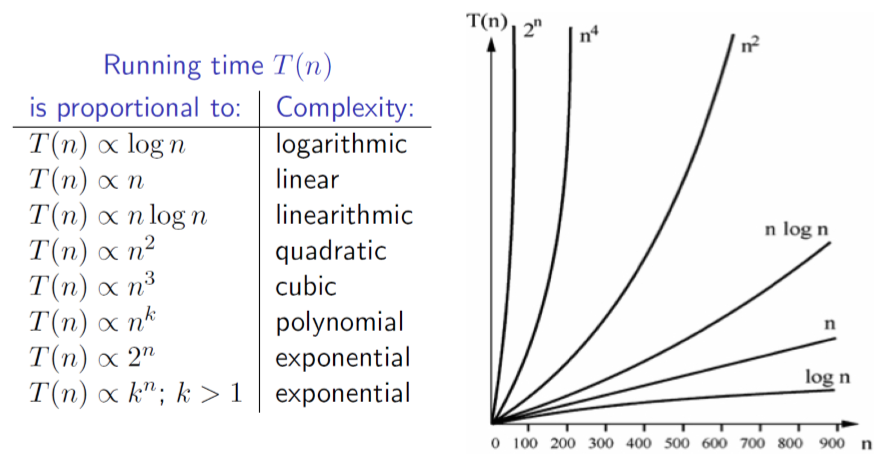
Orders of magnitude
- Order of Magnitude is a mathematical term which basically tells the difference between classes of numbers
- Think of the difference between a room with 10 people, and the same room with 100 people. These are different orders of magnitude
- However, the difference between a room with 100 people and the same room with 101 people is barely noticeable. These are of the same order of magnitude
- How many gumballs in this gumball machine?
- If we guess 200, that’s probably pretty close
- Whereas a guess of 10,000 would be way off

Complexity families
- We will use the following classifications for order of growth (listed by decreasing efficiency, with the most efficient at the top):
- Constant
- Logarithmic ( log(𝑛) )
- Sublinear • Linear (𝑛)
- 𝑛 log(𝑛)
- Polynomial (e.g. 𝑛2, 𝑛3, 𝑛4, etc.)
- Exponential
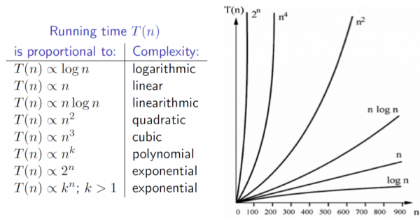
Evaluating complexity
- When evaluating the complexity of an algorithm, keep in mind that you must identify the most expensive computation within an algorithm to determine its classification
- For example, consider an algorithm that is subdivided into two tasks, a task classified as linear followed by a task classified as quadratic. The overall performance of the algorithm must therefore be classified as quadratic
Best, average and worst cases
- As well as the size n of the input, the characteristics of the data in the input set may also have an effect on the time which an algorithm takes to run
- There could be many, many instances of size n which would be valid as input; it may be possible to group these instances into classes with broadly similar features
- Some algorithm “A” may be most efficient overall when solving a given problem. However, it is possible that another algorithm “B” may in fact outperform “A” when solving particular instances of the same problem
- The conclusion to draw is that for many problems, no single algorithm exists which is optimal for every possible input
- Therefore, choosing an algorithm depends on understanding the problem being solved and the underlying probability distribution of the instances likely to be treated, as well as the behaviour of the algorithms being considered.
- Worst case: Defines a class of input instances for which an algorithm exhibits its worst runtime behaviour. Instead of trying to identify the specific input, algorithm designers typically describe properties of the input that prevent an algorithm from running efficiently.
- Average case: Defines the expected behaviour when executing the algorithm on random input instances. While some input problems will require greater time to complete because of some special cases, the vast majority of input problems will not. This measure describes the expectation an average user of the algorithm should have.
- Best case: Defines a class of input instances for which an algorithm exhibits its best runtime behaviour. For these input instances, the algorithm does the least work. In reality, the best case rarely occurs.
Week 3 - Analysing Algorithms Part 2
Analysing Algorithms Part 2
Roadmap
- Review of key concepts
- Complexity
- Orders of growth
- Best, average & worst cases
- Asymptotic notation
- O (Big O)
- Ω (omega)
- Θ (theta)
- Evaluating complexity
- Examples
Review of complexity
- Complexity measures the efficiency of an algorithm’s design, eliminating the effects of platform-specific implementation details (e.g. CPU or complier design)
- We can compare the relative efficiency of algorithms by evaluating their running time complexity on input data of size n (memory or storage requirements of an algorithm could also be evaluated in this manner)
- E.g. how much longer will an algorithm take to execute if we input a list of 1000 elements instead of 10 elements?
- Standard methodology developed over the past half-century for comparing algorithms
- Can determine which algorithms scale well to solve problems of a nontrivial size, by evaluating the complexity the algorithm in relation to the size n of the provided input
- Typically, algorithmic complexity falls into one of a number families (i.e. the growth in its execution time with respect to increasing input size n is of a certain order). The effect of higher order growth functions becomes more significant as the size n of the input set is increased
Comparing growth functions
| value of <m>n</m> | constant | <m>log n</m> | <m>n</m>(linear) | <m>n log n</m>(linearithmic) | <m>n | 2</m>(quadratic) | <m>n | 3</m>(cubic) | <m>2 | n</m>(exponential) |
|---|---|---|---|---|---|---|---|---|---|---|
| 8 | 1 | 3 | 8 | 24 | 64 | 512 | 256 | |||
| 16 | 1 | 4 | 16 | 64 | 256 | 4096 | 65536 | |||
| 32 | 1 | 5 | 32 | 160 | 1024 | 32768 | 4294967296 | |||
| 64 | 1 | 6 | 64 | 384 | 4096 | 262144 | 1.84467E+19 | |||
| 128 | 1 | 7 | 128 | 896 | 16384 | 2097152 | 3.40282E+38 | |||
| 256 | 1 | 8 | 256 | 2048 | 65536 | 16777216 | 1.15792E+77 | |||
| 512 | 1 | 9 | 512 | 4608 | 262144 | 134217728 | 1.3408E+154 |
Best, worst and average cases
- As well as the size n of the input, the actual data that is input may also have an effect on the time which an algorithm takes to run
- There could be many, many instances of size n which would be valid as input; it may be possible to group these instances into classes with broadly similar features
- For many problems, no single algorithm exists which is optimal for every possible input instance
- Therefore, choosing an algorithm depends on understanding the problem being solved and the underlying probability distribution of the instances likely to be encountered, as well as the behaviour of the algorithms being considered
- By knowing the performance of an algorithm under each of these cases, you can judge whether an algorithm is appropriate to use in your specific situation
- Worst case: Defines a class of input instances for which an algorithm exhibits its worst runtime behaviour. Instead of trying to identify the specific input, algorithm designers typically describe properties of the input that prevent an algorithm from running efficiently.
- Average case: Defines the expected behaviour when executing the algorithm on random input instances. While some input problems will require greater time to complete because of some special cases, the vast majority of input problems will not. This measure describes the expectation an average user of the algorithm should have.
- Best case: Defines a class of input instances for which an algorithm exhibits its best runtime behaviour. For these input instances, the algorithm does the least work. In reality, the best case rarely occurs.
Worst case
- For any particular value of n, the number of operations or work done by an algorithm may vary dramatically over all the instances of size n
- For a given algorithm and a given value n, the worst-case execution time is the maximum execution time, where the maximum is taken over all instances of size n
- We are interested in the worst-case behaviour of an algorithm because it often is the easiest case to analyse
- It also explains how slow the program could be in any situation, and provides a lower bound on possible performance
- Good idea to consider worst case if guarantees are required for the maximum possible running time for a given n
- Not possible to find every worst-case input instance, but sample (near) worst-case instances can be crafted given the algorithm’s description
Big O notation
- Big O notation (with a capital latin letter O, not a zero) is a symbolism used in complexity theory, mathematics and computer science to describe the asymptotic behaviours of functions
- In short, Big O notation measures how quickly a function grows or declines
- Also called Landau’s symbol, after the German number theoretician Edmund Landau who invented the notation
- The growth rate of a function is also called its order
- The capitalised greek letter “omicron” was originally used; this has fallen out of favour and the capitalised latin letter “O” is now commonly used
- Example use: Algoroithm X runs in 𝑂(𝑛2) time
- Big O notation is used in computer science to describe the complexity of an algorithm in the worst-case scenario
- Can be used to describe the execution time required or the space used (e.g. in memory or on disk) by an algorithm
- Big O notation can be thought of as a measure of the expected “efficiency” of an algorithm (note that for small sizes of n, all algorithms are efficient, i.e. fast enough to be used for real time applications)
- When evaluating the complexity of algorithms, we can say that if their Big O notations are similar, their complexity in terms of time/space requirements is similar (in the worst case)
- And if algorithm A has a less complex Big O notation than algorithm B, we can infer that it is much more efficient in terms of space/time requirements (at least in the worst case)
Formally
Suppose 𝑓(𝑥) and 𝑔(𝑥) are two functions defined on some subset of the set of real numbers
<m 18>f(x)=O(g(x)) for x right infinity</m>
if and only if there exist constants 𝑁 and 𝐶 such that
<m 18>delim{|}{f(x)}{|}⇐C delim{|}{g(x)}{|} for x all x > N</m>
Intuitively, this means that 𝑓 does not grow more quickly than 𝑔
(Note that N is size of the input set which is large enough for the higher order term to begin to dominate)
Tightest upper bound
- Note that when using Big O notation, we aim to identify the tightest upper bound possible
- An algorithm that is 𝑂(𝑛2) is also 𝑂(𝑛3) , but the former information is more useful
- Specifying an upper bound which is higher than necessary is like saying: “This task will take at most one week to complete”, when the true maximum time to complete the task is in fact five minutes!
Ω (omega) notation
- We can use Ω (omega) notation to describe the complexity of an algorithm in the best case
- Best case may not occur often, but still useful to analyse
- Represents the lower bound on the number of possible operations
- E.g. an algorithm which is Ω 𝑛 exhibits a linear growth in execution time in the best case, as n is increased
Θ (theta) notation
- Finally, Θ (theta) notation is used to specify that the running time of an algorithm is no greater or less than a certain order
- E.g. we say that an algorithm is Θ(𝑛) if it is both O(𝑛) and Ω 𝑛 , i.e. the growth of its execution time is no better or worse than the order specified (linear in this case)
- The actual functions which describe the upper and lower limits do not need to be the exact same in this case, just of the same order
Separating an algorithm and its implementation
- Two concepts:
- The input data size 𝑛, or the number of individual data items in a single data instance to be processed
- The number of elementary operations 𝑓(𝑛) taken by an algorithm, or its running time
- For simplicity, we assume that all elementary operations take the same amount of “time” to execute (not true in practice due to architecture, cache vs. RAM vs. swap/disk access times etc.)
- E.g. an addition, multiplication, division, accessing an array element are all assumed to take the same amount of time
- Basis of the RAM (Random Access Machine) model of computation
- The running time T n of an implementation is: <m>T(n)=c*f(n)</m>
- 𝑓(𝑛) refers to the fact that the running time is a function of the size n of the input dataset
- 𝑐 is some constant
- The constant factor 𝑐 can rarely be determined and depends on the specific computer, operating system, language, compiler, etc. that is used for the program implementation
Evaluating complexity
- When evaluating the complexity of an algorithm, keep in mind that you must identify the most expensive computation within an algorithm to determine its classification
- For example, consider an algorithm that is subdivided into two tasks, a task classified as linear followed by a task classified as quadratic.
- Say the number of operations/execution time is:
- <m>T(n)=50+125n+5n^2</m>
- The overall complexity of the algorithm must therefore be classified as quadratic, we can disregard all lower order terms as the <m>n^2</m> term will become dominant for input sizes of 𝑛=6 or above
- An algorithm with better asymptotic growth will eventually execute faster than one with worse asymptotic growth, regardless of the actual constants
- The actual breakpoint will differ based on the constants and size of the input, but it exists and can be empirically evaluated
- During asymptotic analysis we only need to be concerned with the fastest-growing term of the T(n) function. For this reason, if the number of operations for an algorithm can be computed as <m 13>T(n)=c*n^3+d*n log(n)</m>, we would classify this algorithm as <m 13>O(n^3)</m> because that is the dominant term which grows far more rapidly than <m 13>n log(n)</m>
Passing an array to a method in Java and Python
- If we want to pass multiple values to a method, the easiest way to do this is to pass in an array
- E.g. an array of numbers to be sorted
// passing an array of integers into a method in Java
void myMethod(int[] elements) {
    // do something with the data here
}
def my_function(elements):
    # do something with the data here

test 1 = [5, 1, 12, -5, 16]
my_function(test1)
Array with 5 elements: <m 30>tabular{11}{111111}{5 1 12 {-5} 16}</m>
O(1) example
- O(1) describes an algorithm that will always execute in the same time (or space) regardless of the size of the input data set
- Consider the Java code sample to the right
- No matter how many elements are in the array, this method will execute in constant time
- This method executes in constant time in the best, worst and average cases
Java Code
boolean isFirstElementTwo(int[] elements)
{
    if(elements[0] == 2) {
        return true;
    }
    else {
        return false;
    }
}
Python Code
# O(1) Example
def is_first_el_two(elements):
    if elemenents[0] == 2:
        return True
    return False

test1 = [2, 1, 0, 3]
test2 = [0, 2, 3, 4]

print(is_first_el_two(test1))  # prints True
print(is_first_el_two(test1))  # prints False
O(n) example
- Consider the code samples
- The worst possible time complexity depends linearly on the number of elements in the array
- Execution time for this method is constant in the best case
Java Code
boolean containsOne(int[] elements) {
    for (int i=0; i<elements.size(); i++){
        if(elements[i] == 1) {
            return true;
        }
    }
    return false;
}
Python Code
# O(n) Example
def contains_one(elements)
    for i in range(0, len(elements)):
        if elements[i] == 1:
            return True
    return False

test1 = [0, 2, 1, 2]
test2 = [0, 2, 3, 4]

print(contains_one(test1))  # prints True
print(contains_one(test1))  # prints False
O(n^2) example
- <m>O(n^2)</m> represents an algorithm whose worst case performance is directly proportional to the square of the size of the input data set
- This class of complexity is common with algorithms that involve nested iterations over the input data set (e.g. nested for loops)
- Deeper nested iterations will result in higher orders e.g. <m>O(n^3), O(n^4)</m>, etc.
- Consider the code samples below
- The worst execution time depends on the square of the number of elements in the array
- Execution time for this method is constant in the best case
Java Code
boolean containsDuplicates(int[] elements)
{
  for (int i=0; i<elements.length; i++){
    for (int j=0; j<elements.length; j++){
      if(i == j){ // avoid self comparison continue;
      }
      if(elements[i] == elements[j]) {
        return true; // duplicate found
      }
    }
  }
  return false;
}
Python Code
# O(n^2) Example
def contains_duplicates(elements):
  for i in range (0, len(elements)):
    for j in range(0, len(elements)):
      if i == j: ##avoid self comparison
        continue
      if elements[i] == elements[j]:
        return True # duplicate found
  return False

test1 = [0, 2, 1, 2]
test2 = [1, 2, 3, 4]

print(contains_duplicates(test1))  # prints True
print(contains_duplicates(test2))  # prints False
Week 4 - Recursive Algorithms Part 1
Recursive Algorithms Part 1
Lecture Notes
Socratica Third Part Video
The video and the code is a very condensed summary of the following section and not part of the syllabus, you can skip to Iteration and recursion
Socratica - Recursion, the Fibonacci Sequence and Memoization
Code Summary from the video
- memoization.py
- from functools import lru_cache
- #@lru_cache(maxsize=1000)
- def fibonacci(n):
- if n == 1:
- return 1
- elif n == 2:
- return 1
- elif n > 2:
- return fibonacci(n-1) + fibonacci(n-2)
- for n in range(1, 1001):
- print(n, ":", fibonacci(n))
Run the following code with the highlighted line commented and not commented and observe the difference. The video link above the code explains the details.
Roadmap
- Iteration and recursion
- Recursion traces
- Stacks and recursion
- Types of recursion
- Rules for designing recursive algorithms
Iteration and recursion
- For tasks that must be repeated, up until now we have considered iterative approaches only
- Recap: iteration allows some sequence of steps (or block of code) to be executed repeatedly, e.g using a loop or a while loop
- Recursion is another technique which may be applied to complete tasks which are repetitive in nature
Recursion
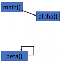
- “Normally”, procedures (or methods) call other procedures
- e.g the main() procedure calls the alpha() procedure
- A recursive procedure is one which calls itself
- e.g the beta() procedure contains a call to beta()
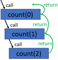
Simple Recursion Program
- you can see that the count method calls itself
- this program would output the values 0 1 2 to the console if run
Java code
void main(){
	count(0);
}

void count(int index){
	print(index);
	if(index <2){
		count(index+1);
	}
}
Python code
def count(index):
  print(index)
  if index < 2:
    count(index + 1)

count(0)    # outputs 0 1 2
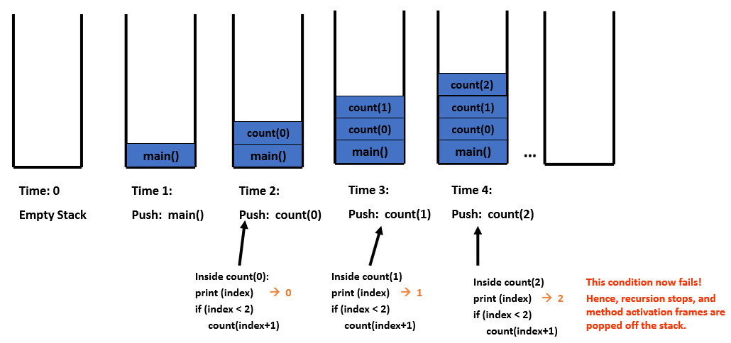
Recursion trace for the call count(0)
Stacks
- A program stack basically operates like a continuer of trays in a cafeteria. It has only two operations:
- Push: push something onto the stack
- Pop: pop something off the top of the stack
- When the method returns or exits, the method’s activation frame is popped off the stack
- Each time a method is invoked, the method’s activation frame (record) is placed on top of the program stack.
Stacks and recursion
Why use recursion?
- with the technique of recursion, a problem may be solved bye solving smaller instances of the same problem
- Some problems are more easily solved by using a recursive approach
- E.g
- Traversing through directories of a file system
- Traversing through a tree of search results
- some sorting algorithms are recursive in nature
- Recursion often leads to cleaner and more concise code which is easier to understand
Recursion vs iteration
- Note: any set of tasks which may be accomplished using a recursive procedure may also be accomplished by using an iterative procedure
- Recursion is “expensive”. The expense of recursion lies in the fact that we have multiple activation frames and the fact that there is overhead involved with calling a method.
- If both of the above statements are true, why would we ever use recursion?
- In many cases, the extra “expense” of recursion is far outweighed by a simpler, clearer algorithm which leads to an implementation that is easier to code.
- Ultimately, the recursion is eliminated when the complier creates assembly language (it does this by implementing the stack)
- If the recursion tree has a simple form, the iterative version may be better
- If the recursion tree appears quite “bushy”, with very few duplicate tasks, then recursion is likely the natural solution
Types of recursion
- Linear recursion: the method makes a single call to itself
- Tail recursion: the method makes a single call to itself, as the last operations
- Binary recursion: the method makes 2 calls to itself
- Exponential recursion: the method makes more than two calls to itself
Tail Recursions
- Tail recustioon is when the last operation in a method is a single recursive call.
- Each time a method is invoked, the method’s activation frame(record) is placed on top of the program stack.
- In this case, there are multiple active stack frames which are unnecessary because they have finished their work.
- Can be expensive and inefficient, so use carefully!
Infinite recursion
- infinite recursion occurs when a recursion method does not have a base case
- consider the method to the right:
- If we call infinite(1), the next call will be infinite(0), then the infinite(-1), then infinite(-2) etc..
- This method will keep making recursive calls to itself until a StackOverflowError occurs (recursive calls have taken up all available memory)
Java code
void infinite(int x){
	infinite(x-1);
}
Pythoncode
def infinite(x):
  infinite(x-1)

infinite(1)
# RecusrionError:
# maximimum recursion depth exceeded
Circular Recursion
- Circular recursion occurs when recursive calls stop making progress towards the base case
- Conside this method
- if we call circular(1), the next call will be circular(2), then the circular(1), then circular(2) etc..
- As with the infinite recursion example, this method will keep making recursive calls to itself until a stack overflow error occurs (recursive calls have taken up all available memory)
Java code
void circular(int x){
	if(x==1){
	  circular(x+1);
	}
	circular(x-1);
}
Python code
def circular(x):
  if x ==1:
    circilar(x + 1)
  circular(x - 1)

circilar(1)    # RecursioError:
# maximum recusrion depth exceeded
# in comparison
Rules for receive algorithms
- Base case: a recursive algorithm must always have a base case which can be solved without recursion. Methods without a base case will results in infinite recursion when run.
- Making progress: for cases that are to be solved recursively, the next recursive call must be a case that makes progress towards the base case. Methods that do not make progress towards the base case will results in circular recursion when run.
- Design rule: Assume that all the recursive calls work.
- Compound interest rule: Never duplicate work by solving the same instance of a problem in separate calls.
Designing Recursive Algorithms
- Think about the task which you wish to accomplish, and try to identify any recurring patterns, e.g. similar operations that must be conducted, like traversing through nested directories on a file system
- Divide the problem up using these recurring operations
- Then
- Identify cases you know can be solved without recursion (base cases). Avoid ending with a multitude of special cases; rather, try to identity a simple base case
- invoke a new copy of the method within each recursion step
- each recursion step resembles the original, larger problem
- Make progress towards the base case(s) with each successive recursive step/call
Recap
- A recursive method is one which calls itself within its method body
- Recursion allows us to solve a problem, by breaking it up into smaller instances of the same problem
- Recursive methods must always have a base case which may be solved without recursion
- In the next lecture we will consider some example problems which may be solved using recursion
Week 5 - Recursive Algorithms Part 2
Roadmap
- Review of recursion
- Sample recursive algorithms
- Factorials
- Greatest common divisor
- Fibonacci series
Review of recursion
- “Normally”, procedures (or methods) call other procedures
- e.g the main() procedure calls the alpha() procedure
- A recursive procedure is one which calls itself
- e.g the beta() procedure contains a call to beta()
Rules for recursive algorithms
- Base case: a recursive algorithm must always have a base case which can be solved without recursion. Methods without a base case will result in infinite recursion when run.
- Making progress: for cases that are to be solved recursively, the next recursive call must be a case that makes progress towards the base case. Methods that do not make progress towards the base case will result in circular recursion when run.
- Design rule: assume that all the recursive call work
- Compound interest rule: Never duplicate work by solving the same instance of a problem in separate recursive calls.
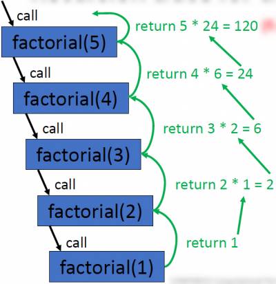
Factorials
- The factorial of a non-negative integer n may be computed as the product of all positive integers which are less than or equal to n
- This is denoted by n!
- in general : n! = n * (n-1)* (n-2)*(n-3)*….*1
- The above is essentially an algorithm which may be implemented and used to calculate the factorial of any n >0
- Note: the value of 0! is defined as 1 ( i.e 0! = 1 following the empty product convention), The input n=0 will serve as the base case in our recursive implementation
- Factorial operations are commonly used in many areas of mathematics, e.g combinatorics, algebra, computation of functions such as sin and cos, and the binomial theorem.
- One of its most basic occurrences is the fact that there are n! ways to arrange distinct objects into a sequence
- In general: n! = n *(n - 1)*(n-2)*(n-3)*..*1
- Example factorial calculation: 5! = 5*4*3*2*1 = 120
Computing a factorial
iterative implementation
def factorial(n):
	answer = 1
	while n > 1:
		answer *= n
		n -=1
	return answer

print(factorial(5))
#prints 120
Recursive implementation
def factorial_rec(n):
	if n <1:
		return 1
	else:
		return n*factorial_rec(n-1)

print(factorial_rec(5))
#print 120
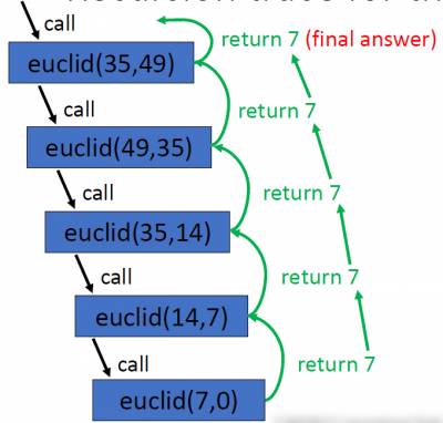
Greatest common Divisor
- The greatest common divisor (gcd) of two integer is the largest positive integer which divides into both numbers without leaving a remainder
- e.g the gcd of 30 and 35 is 5
- Euclid’s algorithm (c. 300 BC) may be used to determine the gcd of two integers
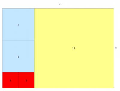
- Example application: finding the largest square tile which can be used to cover the floor of a room without using partial/cut tile
Computing the greatest common divisor
iterative implementation
def euclid(a, b):
	while b != 0:
		temp = b
		b = a% b
		a = temp
	return a

print(euclid(35, 49))
# print 7
Recursive implementation
def euclid (a, b):
	if b == 0:
		return a
	else:
		return euclid(b, a%b)
print(euclid(35, 49))
# prints 7
Fibonacci series
- 0,1,1,2,3,5,8,13,21,34,55,89,144,233,377,610
- the Fibonacci series crops up very often in nature and can be used to model the growth rate of organisms
- e.g leaf arrangements in plants, numbers of petals on a flower, the bracts of a pinecone, the scales of pineapple, shells, proportions of the human body
- The fibonacci series is named after the Italian mathematician Leonardo of Pisa, who was also known as Fibonacci
- His book Liber Abaci (published 1202) introduced the sequence to western world (Indian mathematicians knew about this sequence previously).
- We will use the convention that zero is included in the series and assigned to index 1
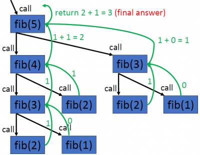
- if fib(n) is a method that returns the nth number in the series, then: fib(1)=0, fib(2)=1, fib(3)=1, fib(4)=2, fib(5)=3, fib(6)=5, fib(7)=8, etc…
- In general, fib(n) = fib(n-1) +fib(n-2)
- The results for fib(1) and fib(2) do not conform to this rule; therefore they will serve as base cases in our recursive implementation
Computing the nth Fibonacci number
Iterative implementation
def fib(n):
	i, n1, n2 =1, 0, 1
	while i <n:
		temp =n1
		n1 = n2
		n2 =n1 +temp
		i = 1+ i
	return n1

print(fib(5))
#prints 3
Recursive implementation
def fib(n):
	if n==1:
		return 0
	elif n ==2:
		return 1
	return fib(n-1) +fib(n-2)

print(fib(5))
#prints 3
Week 6 - Cryptography
Overview
07_algorithms_cryptography_ssl_2019_part1.pdf
- Crytography (terms and definitions)
- Types of cry–systems (symmetric and asymmetric)
- Examples of systems in practice
Introduction to Cryptography
- Cryptography is the science of secrecy and is concerned with the need to communicate in secure, private and reliable ways
- From a computational thinking/algorithmics perspective, a novel feature is the fact (as we will see ) that modern methods used to solve cryptographic problems exploit the difficulty of solving other problems.
This is somewhat surprising…..
problems for which no good algorithms are known are crucial here.
Cryptography (Problem Statement)
- The basic problem to be solved is that of encrypting and decrypting data.
- How should we encode an important message in such a way that the receiver should be able to decipher it, but not an eavesdropper?
- Moreover, can then message be signed by the sender so that:
- The receiver can be sure that only the sender could have sent it.
- The sender cannot later deny having sent it
- The receiver, having received the signed message, cannot sign a message in the sender name, not even additional versions of the very message that has just been received.
Cryptography (Some definitions)
- Data that can be read and understood without any special measure is called plaintext(or clear text). Plaintext, P, is the input to an encryption process(algorithm).
- Encryption is the process of disguising plaintext in such a way as to hide its substance.
- The result (output..) of the encryption process is ciphertext, C
A general encryption procedure(left ) and decryption procedure (right) is as follows:
<m 20>C = Encr(P)</m> and <m 20>P = Decr(C)</m>

Symmetric Cryptography
- In conventional cryptography, also called secret-key or symmetric-key encryption, one key is used both for encryption and decryption
- EG. The data Encryption Standard (DES) cryptosystem
Symmetric Cryptography - Simple Example
Substitution Cipher
- The Caesar cipher shifted the alphabet by 3 characters

EG: Hello - > khoor
- Caesar cipher is a one to one mapping. A mono alphabetic substitution!
- Cryptanalysis exploits statistical properties of the English language.
- “E” is the most frequently occurring letter

So from example above, this kind of cypher is easily broken…
Symmetric Cryptography - Examples continued...
Polyalphabetic substitution:
- The key is a simple phrase of fixed length(which can repeat).
- Add the value of the letter in the key to the value of the letter inthe plaintext to ciphertext, and “wrap around” if necessary (modulo 36)

- This is essentially multiple Caesar-type ciphers
- Main advantage is that same plaintext get mapped onto different cipher-text.
Polyalphabetic substitution continued

- This is essentially multiple Caesar-type ciphers
- Main advantage is that same plaintext get mapped onto different ciphertext


Decryption Algorithm


Cryptography: Algorithms and keys
- The strength of a cryptosystem is a function of:
- The strength of the algorithm
- The length (or size) of the key
- The assumption is that the general method of encryption (i.e the algorithm is known), and the security of the system lies in the secrecy of the key.
- eg: General idea of a combination pad lock is known, strength is in secret combination.
- The larger the key, the higher the work factor for the cryptanalyst.
- A brute-force attack means trying all possible key values.
Cryptographic keys
- In our earlier example, we had a phrase as our key to unlocking the secret message:

…and each letter of the phrase could take on 1 of 26 possible numeric values.
Ours are (t =20, h= 8 etc…)

As we had 10 characters in our phrase, and each character could be any 1 of 26 possible values, our potential key space is <m>26^10</m> i.e there are 141,167,095,653,376 possible keys or “phrases”.

- Let's think of key as multiples of bits or bytes in a computer system
- If a key is 8 bits long, then there are 2^8 = 256 possible keys
- A key that is 56-bits long has 2^56 possible key values. A very large number!
- *72,057,594,927,936 possible values in fact! * If a computer could try one million keys per second, it would take over 2000 years to try all key values.*
- 72, 057, 594, 927, 936 possible values @1,0000,000
- 72,057,594,037,927,936/1,000,000 = 72057594037 seconds required to test all values
- 72057594037/60 = 1,200,959,900 minutes required to test all values
- 1,200,959,900/60 = 20,015,998.33 hours required to test all values
- 20,015,998.33/24 = 833,999.93 days required to test all values/365 = 2,284 YEARS
- If a 64-bit key were used, it would take 600,000 years to try all possible key values (at a test rate 1 million keys per second)
- For a 128-bit key, it would take 10^25 years. The universe is only 10^10 years old.
- When trying a brute force attack need to consider:
- Number of keys to be tested
- The speed of each test
Some limitations of Symmetric Cryptography
- Consider our problem statement from earlier (which outlined what our desired solution should solve)

- Does not address the signature issue…
- Receiver could make up fake messages?
- Sender could deny having sent authentic messages
- Another major drawback (particularly in a distributed environment like the internet) is the issue of key distribution and management
- Symmetric systems require parties to cooperate in the generation an distribution of key pairs. Not scalable (even where it might be “culturally” feasible)
Cryptography: Key Distribution
- Ciphers have improved significantly in terms of complexity since the days of Caesar. However….
- As noted, a big issue with symmetric cryptographic systems is that of Key management; specifically with respect to transferring keys.
- How do the sender and receiver agree on the same key?
- split the key into several parts?
- Other…?
Asymmetric Cryptography: Public Key Cryptography
- The problems of key distribution are solved by public key cryptography
- Public key cryptography is an asymmetric scheme that uses a pair of keys for encryption: a public key, which encrypts data, and a corresponding private, or secret key for decryption.
- You publish you public key to the world while keeping your private key secret. Anyone with a copy of your public key can then encrypt information that only you can read.
- Crucially, it is computationally infeasible to deduce the private key from the public key
Public Key Cryptography
- The primary benefit of public key crptograohy is that it allows people who have no pre-existing security arrangement to exchange messages securely.

- The need for sender and receiver to share secret keys via some secure channel is eliminated; all communications involve only public keys, and no private key is ever transmitted or shared.
A little bit of number theory
Prime number: A number is prime if it is greater than 1 and if its only factors are itself and 1.
- 1 is not prime (1 is not greater than 1)
- 2 is prime (the only even prime)
- 3 is prime
- 4 is not prime (no other even number - except 2 - is prime)…4 *1, 2*2
- 5 is prime (but being odd does not necessarily make you prime)
- 6 is not prime 6*1, 3*2
- 8 is not prime…8*1, 2*4
- 9 is not prime (but it is odd)…9*1, 3*3
RSA Algorithm
- First published in 1978 (and still secure) (researchers: Ron Rivet, Adi Shamir, Len Adleman)
- A block ciphering scheme, where the plaintext and cipher-text are integers between 0 and -1, for some value n.
(Foundation is a number theory in mathematics, based on Euler's generalisation of Fermat's Theorem).
Format
A block of plaintext(message), M, gets transformed into a cipher block C

- Both sender and receiver know the value of n (public)
- sender/everyone knows the value of e (public)
- Receiver only knows the value of d (Private)

Requirements:

RSA: A (simple) example
- Suppose I wish to send my access number securely across an “open” network.
e.g. PIN = 2345
- I don't want my account to be hacked; neither does my employer!
- My employer implements a security system (based on the RSA algorithm, for instance) and tells me (and everyone else)….
“When sending us private data such as your PIN, encrypt it using RSA. This is the relevant public key information: e=7, n=33”
Encrypting my "Plaintext" PIN: 2 3 4 5


- An “attacker” listening in on the connection might capture your encrypted PIN (i.e they could discover 29,9,16,14)
- Furthermore they would know that this is the output of the known RSA algorithm (C = P^e mod n)
- …They would know that e=7 and that n = 33 as these are publicly available)
- But… they won't be able to figure out P (the plaintext) in a reasonable amount of time
Decrypting 29,9,16,14
- Can only be done (in a reasonable amount of time) if you know the private/secret, d
- d is not publicly available and is jealously guarded by the owner.
- Decryption is straightforward if you know the value of d.

- Raising the ciphertext to the power of d, modulo n, will give you back the plaintext.


- Note that a knowledges of the encryption algorithm, a knowledge of the encryption key and a copy of the ciphertext is not sufficient to get back the plaintext (in a reasonable amount of time)
- You must also know the value of d, the private key.
- The beauty of RSA is that the encryption key and process can be made public without compromising the security of the system. This solves the “Key distribution” problem outlined earlier.
Next steps
- Future session to look at RSA in more detail including some of the underpinnings of the algorithm.
- Authentication and signatures using RSA
- Secure Sockets Layer(SSL) Algorithm
- RSA performance
- Attacking RSA
To do W6
- Contribute to the discussion forum on Moodle/LearnOnline
- Further reading in this area
| DATA ANALYTICS REFERENCE DOCUMENT |
|
|---|---|
| Document Title: | Document Title |
| Document No.: | 1552735583 |
| Author(s): | Gerhard van der Linde, Rita Raher |
| Contributor(s): | |
REVISION HISTORY
| Revision | Details of Modification(s) | Reason for modification | Date | By |
|---|---|---|---|---|
| 0 | Draft release | Document description here | 2019/03/16 11:26 | Gerhard van der Linde, Rita Raher |
Week 8 - Sorting Algorithms Part 1
Overview
- Introduction to sorting
- Conditions for sorting
- Comparator functions and comparison-based sorts
- Sort keys and satellite data
- Desirable properties for sorting algorithms
- Stability
- Efficiency
- In-place sorting
- Overview of some well-known sorting algorithms
- Criteria for choosing a sorting algorithm
Sorting
- Sorting – arrange a collection of items according to some pre-defined ordering rules
- There are many interesting applications of sorting, and many different sorting algorithms, each with their own strengths and weaknesses.
- It has been claimed that as many as 25% of all CPU cycles are spent sorting, which provides a great incentive for further study and optimization
- The search for efficient sorting algorithms dominated the early days of computing.
- Numerous computations and tasks are simplified by properly sorting information in advance, e.g. searching for a particular item in a list, finding whether any duplicate items exist, finding the frequency of each distinct item, finding order statistics of a collection of data such as the maximum, minimum, median and quartiles.
Timeline of sorting algorithms
- 1945 – Merge Sort developed by John von Neumann
- 1954 – Radix Sort developed by Harold H. Seward
- 1954 – Counting Sort developed by Harold H. Seward
- 1959 – Shell Sort developed by Donald L. Shell
- 1962 – Quicksort developed by C. A. R. Hoare
- 1964 – Heapsort developed by J. W. J. Williams
- 1981 – Smoothsort published by Edsger Dijkstra
- 1997 – Introsort developed by David Musser
- 2002 – Timsort implemented by Tim Peters
Sorting
- Sorting is often an important step as part of other computer algorithms, e.g. in computer graphics (CG) objects are often layered on top of each other; a CG program may have to sort objects according to an “above” relation so that objects may be drawn from bottom to top
- Sorting is an important problem in its own right, not just as a preprocessing step for searching or some other task
- Real-world examples:
- Entries in a phone book, sorted by area, then name
- Transactions in a bank account statement, sorted by transaction number or date
- Results from a web search engine, sorted by relevance to a query string
Conditions for sorting
- A collection of items is deemed to be “sorted” if each item in the collection is less than or equal to its successor
- To sort a collection A, the elements of A must be reorganised such that if A[i] < A[j], then i < j
- If there are duplicate elements, these elements must be contiguous in the resulting ordered collection – i.e. if A[i] = A[j] in a sorted collection, then there can be no k such that i < k < j and A[i] ≠ A[k].
- The sorted collection A must be a permutation of the elements that originally formed A (i.e. the contents of the collection must be the same before and after sorting)
Comparing items in a collection
- What is the definition of “less than”? Depends on the items in the collection and the application in question
- When the items are numbers, the definition of “less than” is obvious (numerical ordering)
- If the items are characters or strings, we could use lexicographical ordering (i.e. apple < arrow < banana)
- Some other custom ordering scheme – e.g. Dutch National Flag Problem (Dijkstra), red < white < blue
Comparator functions
- Sorting collections of custom objects may require a custom ordering scheme
- In general: we could have some function compare(a,b) which returns:
- -1 if a < b
- 0 if a = b
- 1 if a > b
- Sorting algorithms are independent of the definition of “less than” which is to be used
- Therefore we need not concern ourselves with the specific details of the comparator function used when designing sorting algorithms
Inversions
- The running time of some sorting algorithms (e.g. Insertion Sort) is strongly related to the number of inversions in the input instance.
- The number of inversions in a collection is one measure of how far it is from being sorted.
- An inversion in a list A is an ordered pair of positions (i, j) such that:
- i < j but A[i] > A[j].
- i.e. the elements at positions i and j are out of order
- E.g. the list [3,2,5] has only one inversion corresponding to the pair (3,2), the list [5,2,3] has two inversions, namely, (5,2) and (5,3), the list [3,2,5,1] has four inversions (3,2), (3,1), (2,1), and (5,1), etc.
Comparison sorts
- A comparison sort is a type of sorting algorithm which uses comparison operations only to determine which of two elements should appear first in a sorted list.
- A sorting algorithm is called comparison-based if the only way to gain information about the total order is by comparing a pair of elements at a time via the order ≤.
- Many well-known sorting algorithms (e.g. Bubble Sort, Insertion Sort, Selection Sort, Merge Sort, Quicksort, Heapsort) fall into this category.
- Comparison-based sorts are the most widely applicable to diverse types of input data, therefore we will focus mainly on this class of sorting algorithms
- A fundamental result in algorithm analysis is that no algorithm that sorts by comparing elements can do better than <m>n</m> log <m>n</m> performance in the average or worst cases.
- Under some special conditions relating to the values to be sorted, it is possible to design other kinds of non-comparison sorting algorithms that have better worst-case times (e.g. Bucket Sort, Counting Sort, Radix Sort)
Sort keys and satellite data
- In addition to the sort key (the information which we use to make comparisons when sorting), the elements which we sort also normally have some satellite data
- Satellite data is all the information which is associated with the sort key, and should travel with it when the element is moved to a new position in the collection
- E.g. when organising books on a bookshelf by author, the author’s name is the sort key, and the book itself is the satellite data
- E.g. in a search engine, the sort key would be the relevance (score) of the web page to the query, and the satellite data would be the URL of the web page along with whatever other data is stored by the search engine
- For simplicity we will sort arrays of integers (sort keys only) in the examples, but note that the same principles apply when sorting any other type of data
Desirable properties for sorting algorithms
- Stability – preserve order of already sorted input
- Good run time efficiency (in the best, average or worst case)
- In-place sorting – if memory is a concern
- Suitability – the properties of the sorting algorithm are well-matched to the class of input instances which are expected i.e. consider specific strengths and weaknesses when choosing a sorting algorithm
Stability
- If a comparator function determines that two elements 𝑎𝑖 and 𝑎𝑗 in the original unordered collection are equal, it may be important to maintain their relative ordering in the sorted set
- i.e. if i < j, then the final location for A[i] must be to the left of the final location for A[j]
- Sorting algorithms that guarantee this property are stable
- Unstable sorting algorithms do not preserve this property
- Using an unstable sorting algorithm means that if you sort an already sorted array, the ordering of elements which are considered equal may be altered!
Stable sort of flight information
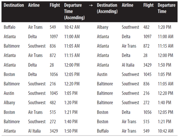
- All flights which have the same destination city are also sorted by their scheduled departure time; thus, the sort algorithm exhibited stability on this collection.
- An unstable algorithm pays no attention to the relationships between element locations in the original collection (it might maintain relative ordering, but it also might not).
Reference: 1)
Analysing sorting algorithms
- When analysing a sorting algorithm, we must explain its best-case, worstcase, and average-case time complexity.
- The average case is typically hardest to accurately quantify and relies on advanced mathematical techniques and estimation. It also assumes a reasonable understanding of the likelihood that the input may be partially sorted.
- Even when an algorithm has been shown to have a desirable best-case, average-case or worst-case time complexity, its implementation may simply be impractical (e.g. Insertion Sort with large input instances).
- No one algorithm is the best for all possible situations, and so it is important to understand the strengths and weaknesses of several algorithms.
Recap: orders of growth
Factors which influence running time
- As well as the complexity of the particular sorting algorithm which is used, there are many other factors to consider which may have an effect on running time, e.g.
- How many items need to be sorted
- Are the items only related by the order relation, or do they have other restrictions (for example, are they all integers in the range 1 to 1000)
- To what extent are the items pre-sorted
- Can the items be placed into an internal (fast) computer memory or must they be sorted in external (slow) memory, such as on disk (so-called external sorting).
In-place sorting
- Sorting algorithms have different memory requirements, which depend on how the specific algorithm works.
- A sorting algorithm is called in-place if it uses only a fixed additional amount of working space, independent of the input size.
- Other sorting algorithms may require additional working memory, the amount of which is often related to the size of the input n
- In-place sorting is a desirable property if the availability of memory is a concern
Overview of sorting algorithms
| Algorithm | Best case | Worst case | Average case | Space Complexity | Stable? | |||
|---|---|---|---|---|---|---|---|---|
| Bubble Sort | <m>n</m> | <m>n | 2</m> | <m>n | 2</m> | 1 | Yes | |
| Selection Sort | <m>n | 2</m> | <m>n | 2</m> | <m>n | 2</m> | 1 | No |
| Insertion Sort | <m>n</m> | <m>n | 2</m> | <m>n | 2</m> | 1 | Yes | |
| Merge Sort | <m>n log n</m> | <m>n log n</m> | <m>n log n</m> | <m>O(n)</m> | Yes | |||
| Quicksort | <m>n log n</m> | <m>n | 2</m> | <m>n log n</m> | <m>n</m> (worst case) | No* | ||
| Heapsort | <m>n log n</m> | <m>n log n</m> | <m>n log n</m> | 1 | No | |||
| Counting Sort | <m>n + k</m> | <m>n + k</m> | <m>n + k</m> | <m>n + k</m> | Yes | |||
| Bucket Sort | <m>n + k</m> | <m>n | 2</m> | <m>n + k</m> | <m>n * k</m> | Yes | ||
| Timsort | <m>n</m> | <m>n log n</m> | <m>n log n</m> | <m>n</m> | Yes | |||
| Introsort | <m>n log n</m> | <m>n log n</m> | <m>n log n</m> | <m>log n</m> | No |
*the standard Quicksort algorithm is unstable, although stable variations do exist
Criteria for choosing a sorting algorithm
| Criteria | Sorting algorithm |
|---|---|
| Small number of items to be sorted | Insertion Sort |
| Items are mostly sorted already | Insertion Sort |
| Concerned about worst-case scenarios | Heap Sort |
| Interested in a good average-case behaviour | Quicksort |
| Items are drawn from a uniform dense universe | Bucket Sort |
| Desire to write as little code as possible | Insertion Sort |
| Stable sorting required | Merge Sort |
Week 9: Sorting Algorithms Part 2
Overview
- Review of sorting & desirable properties for sorting algorithms
- Introduction to simple sorting algorithms
- Bubble Sort
- Selection sort
- Insertion sort
Review of sorting
- Sorting - Arrange a collection of items according to pre-defined ordering rule
- Desirable properties for sorting algorithms
- Stability - preserve order of already sorted input
- Good run time efficiency(in the best, average or worst case)
- In-place sorting - if memory is a concern
- Suitability - the properties of the sorting algorithm are well-matched to the class of input instances which are expected i.e. consider specific strengths and weaknesses when choosing a sorting algorithm.
Overview of sorting algorithms
| Algorithm | Best case | Worst case | Average case | Space Complexity | Stable? | |||
|---|---|---|---|---|---|---|---|---|
| Bubble Sort | <m>n</m> | <m>n | 2</m> | <m>n | 2</m> | 1 | Yes | |
| Selection Sort | <m>n | 2</m> | <m>n | 2</m> | <m>n | 2</m> | 1 | No |
| Insertion Sort | <m>n</m> | <m>n | 2</m> | <m>n | 2</m> | 1 | Yes | |
| Merge Sort | <m>n log n</m> | <m>n log n</m> | <m>n log n</m> | <m>O(n)</m> | Yes | |||
| Quicksort | <m>n log n</m> | <m>n | 2</m> | <m>n log n</m> | <m>n</m> (worst case) | No* | ||
| Heapsort | <m>n log n</m> | <m>n log n</m> | <m>n log n</m> | 1 | No | |||
| Counting Sort | <m>n + k</m> | <m>n + k</m> | <m>n + k</m> | <m>n + k</m> | Yes | |||
| Bucket Sort | <m>n + k</m> | <m>n | 2</m> | <m>n + k</m> | <m>n * k</m> | Yes | ||
| Timsort | <m>n</m> | <m>n log n</m> | <m>n log n</m> | <m>n</m> | Yes | |||
| Introsort | <m>n log n</m> | <m>n log n</m> | <m>n log n</m> | <m>log n</m> | No |
*the standard Quicksort algorithm is unstable, although stable variations do exist
Comparison sorts
- A comparison sort is a type of sorting algorithm which uses comparison operations only to determine which of two elements should appear in a sorted list.
- A sorting algorithm is called comparison-based if the only way to gain information about the total order is by comparing a pair of elements at a time via the order ≤
- The simple sorting algorithms which we will discuss in this lecture (Bubble sort, insertion sort, and selection sort) all fall into this category.
- A fundamental result in algorithm analysis is that no algorithm that sorts by comparing elements can do better than <m>n</m> log <m>n</m> performance in the average or worst cases.
- Non-comparison sorting algorithms(e.g Bucket Sort, Counting Sort, Radix Sort) can have better worst-case times.
Bubble Sort
- Named for the way larger values in a list “Bubble up” to the end as sorting takes place
- Bubble sort was first analysed as early as 1956 (time complexity is <m>n</m> in best case, and <m>n^2</m> in worst and average cases)
- Comparison-based
- In-place sorting algorithm(i.e uses a constant amount of additional working space in addition to the memory required for the input)
- Simple to understand and implement, but it is slow and impractical for most problems even when compared to Insertion sort.
- Can be practical in some cases on data which is nearly sorted
Bubble Sort procedure
- Compare each element(except the last one) with its neighbour to the right
- if they are out of order, swap them
- this puts the largest element at the very end
- the last element is now in the correct and final place
- Compare each element(except the last two) with its neighbour to the right
- If they are out of order, swap them
- This puts the second largest element next to last
- The last two elements are now in their correct and final places.
- Compare each element (except the last three) with its neighbour to the right
- …
- Continue as above until there are no unsorted elements on the left
Bubble Sort example

Bubble Sort in Code
public static void bubblesort(int[]a){
  int outer, inner;
  for(outer = a.length - 1; outer > 0;outer--){ //counting down
   for(inner=0;inner < outer;inner++){ //bubbling up
    if(a[inner] > a[inner+1];  { //if out of order....
    int temp = a[inner]; //...then swap
    a[inner] =a[inner+1];
    a[inner +1] = temp;
    }
   }
  }
 }
- bubblesort.py
# Bubble Sort in python
def printArray(arr):
  print (' '.join(str(i) for i in arr))


def bubblesort(arr):
  for i in range(len(arr)):
    for j in range(len(arr) - i - 1):
      if arr[j] > arr[j + 1]:
        temp = arr[j]
        arr[j] = arr[j + 1]
        arr[j + 1] = temp
    # Print array after every pass
    print ("After pass " + str(i) + "  :", printArray(arr))

if __name__ == '__main__':
    arr = [10, 7, 3, 1, 9, 7, 4, 3]
    print ("Initial Array :", printArray(arr))
    bubblesort(arr)
Bubble Sort Example

Analysing Bubble Sort (worst case)
for(outer =a.length-1; outer >0; outer--){
 for(inner=0; inner < outer; inner++){
  if(a[inner]>a[inner+1]){
  //swap code omitted
  }
 }
}
- In the worst case, the outer loop executes n-1 times (say n times)
- On average, inner loop executes about n/2 times for each outer loop
- In the inner loop, comparison and swap operations take constant time k
- Result is:

Selection Sort
- Comparison-based
- In-place
- Unstable
- Simple to implement
- Time complexity is <m>n^2</m> in best, worst and average cases.
- Generally gives better performance than Bubble Sort, but still impractical for real world tasks with a significant input size
- In every iteration of selection sort, the minimum element (when ascending order) from the unsorted subarray on the right is picked and moved to the sorted subarray on the left.
Selection Sort procedure
- Search elements 0 through n-1 and select the smallest
- swap it with the element in location 0
- Search elements 1 through n-1 and select the smallest
- swap it with the element in location 1
- Search elements 2 through n-1 and select the smallest
- swap it with the element in location 2
- Search elements 3 through n-1 and select the smallest
- swap it with the element in location 3
- Continue in this fashion until there's nothing left to search
Selection Sort example

The element at index 4 is the smallest, so swap with index 0
The element at index 2 is the smallest, so swap with index 1
The element at index 3 is the smallest, so swap with index 2
The element at index 3 is the smallest, so swap with index 3
Selection sort might swap an array element with itself; this is harmless, and not worth checking for
Selection Sort in Code
public static void selectionsort(int[]a){
 int outer=0, inner=0, min=0;
 for(outer = 0; outer <a.length-1;outer++){  //outer counts up
 min = outer;
 for(inner = outer +1; inner <a.length; inner++){
  if(a[inner]<a[min]){ //find index of smallest value
   min = inner;
   }
  }
  //swap a [min] with a [outer]
  int temp = a[outer];
  a[outer] = a[min];
  a[min] = temp;
 }
}
- selection_sort.py
# selection sort in python
def printArray(arr):
  return (' '.join(str(i) for i in arr))


def selectionsort(arr):
  N = len(arr)
  for i in range(0, N):
    small = arr[i]
    pos = i
    for j in range(i + 1, N):
      if arr[j] < small:
        small = arr[j]
        pos = j
    temp = arr[pos]
    arr[pos] = arr[i]
    arr[i] = temp
    print ("After pass " + str(i) + "  :", printArray(arr))

if __name__ == '__main__':
    arr = [10, 7, 3, 1, 9, 7, 4, 3]
    print ("Initial Array :", printArray(arr))
    selectionsort(arr)
Analysing Selection Sort

- The outer loop runs <m>n</m> - 1 times
- The inner loop executes about <m>n</m>/2 times on average(from <m>n</m> to 2 times)
- Results is:
 in best, worst and average cases
Insertion Sort
- Similar to the method usually used by card players to sort cards in their hand.
- Insertion sort is easy to implement, stable, in-place, and works well on small lists and lists that are close to sorted.
- On data sets which are already substantially sorted it runs in n +d time, where d is the number of inversions.
- However, it is very inefficient for large random lists.
- Insertion Sort is iterative and works by splitting a list of size n into a head(“sorted”) and tail(“unsorted”) sublist.
Insertion Sort procedure
- Start from the left of the array, and set the “key” as the element at index 1.Move any elements to the left which are > the “key” right by one position, and insert the “key”.
- Set the “Key” as the element at index 2. Move any elements to the left which are > the key right by one position and insert the key.
- Set the “key” as the element at the index 3. Move any elements to the left which are > the key right by one position and index the key.
- …
- Set the “key” as the elements at index <m>n</m>-1. Move any elements to the left which are > the key right by one position and insert the key.
- The array is now sorted.
Insertion Sort example

a[1]=5 is the key; 7>5 so move 7 right by one position, and insert 5 at index 0
a[2]=2 is the key; 7>2 so move both 7 and 5 right by one position, and insert 2 at index 0
a[3]=3 is the key; 7>3 and 5>3 so move both 7 and 5 right by one position, and insert 3 at index 1
a[4]=1 is the key; 7>1, 5>1, 3>1 and 2>1 so move both 7, 5, 3 and 2 right by one position, and insert 1 at index 1
(done)
Insertion Sort in code
public static void insertionsort(int a[]){
 for(int i=1; i<a.length; i++){
  int key =a[i]; //value to be inseted
  int j = i-1;
  //move all elements > key right one position
  while(j>=0 && a[j]>key){
  a[j+1]= a[j];
  j=j-1;
  }
  a[j+1]=key; //insert key in its new position
 }

}
- insertion_sort.py
# insertion sort
def printArray(arr):
  return(' '.join(str(i) for i in arr))


def insertionsort(arr):
  N = len(arr)
  for i in range(1, N):
    j = i - 1
    temp = arr[i]
    while j >= 0 and temp < arr[j]:
      arr[j + 1] = arr[j]
      j -= 1
    arr[j + 1] = temp
    print ("After pass " + str(i) + "  :", printArray(arr))

if __name__ == '__main__':
    arr = [10, 7, 3, 1, 9, 7, 4, 3]
    print ("Initial Array :", printArray(arr))
    insertionsort(arr)
Analysing Insertion Sort
- The total number of data comparisons made by insertion sort is the number of inversions d plus at most <m>n</m> -1
- A sorted list has no inversions - therefore insertion sort runs in linear Ω(n) time in the best case(when the input is already sorted)
- On average, a list of size <m>n</m> has
 inversions, and the number of comparisons is
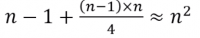
- In the worst case, alist of size n has
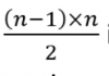 inversions(reserve sorted input), and the number of comparisons is
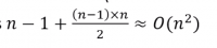


Comparison of Simple sorting algorithms
- The main advantage that Insertion sort has over Selection Sort is that the inner loop only iterates as long as is necessary to find the insertion point.
- In the worst case, it will iterate over the entire sorted part. In the case, the number of iterations is the same as for selection sort and bubble sort.
- At the other extreme, however, if the array is already sorted, the inner loop won't need to iterate at all. In this case, the running time is Ω(n), which is the same as the running time of Bubble sort on an array which is already sorted.
- Bubble Sort, Selection sort and insertion sort are all in-place sorting algorithms.
- Bubble sort and insertion sort are stable, whereas selection sort
Criteria for choosing a sorting algorithm
| Criteria | Sorting algorithm |
|---|---|
| Small number of items to be sorted | Insertion Sort |
| Items are mostly sorted already | Insertion Sort |
| Concerned about worst-case scenarios | Heap Sort |
| Interested in a good average-case behaviour | Quicksort |
| Items are drawn from a uniform dense universe | Bucket Sort |
| Desire to write as little code as possible | Insertion Sort |
| Stable sorting required | Merge Sort |
Recap
- Bubble sort, selection sort and insertion sort are all O(<m>n^2</m>) in the worst case
- It is possible to do much better than this even with comparison-based sorts, as we will see in the next lecture
- from this lectuure on simple O(<m>n^2</m>)sorting algorithms:
- Bubble sort is extremely slow, and is of little practical use
- Selection sort is generally better than Bubble sort
- Selection sort and insertion sort are “good enough” for small input instances
- Insertion sort is usually the fastest of the three. In fact, for small <m>n</m> (say 5 or 10 elements), insertion sort is usually fasters than more complex algorithms.
Week 10: Sorting Algorithms Part 3
Overview
- Efficient comparison sort
- Merge sort
- Quick sort
- Non-comparison sorts
- Counting sort
- Bucket sort
- Hybrid Sorting algorithms
- Introsort
- Timsort
Overview of sorting algorithms
| Algorithm | Best case | Worst case | Average case | Space Complexity | Stable? | |||
|---|---|---|---|---|---|---|---|---|
| Bubble Sort | <m>n</m> | <m>n | 2</m> | <m>n | 2</m> | 1 | Yes | |
| Selection Sort | <m>n | 2</m> | <m>n | 2</m> | <m>n | 2</m> | 1 | No |
| Insertion Sort | <m>n</m> | <m>n | 2</m> | <m>n | 2</m> | 1 | Yes | |
| Merge Sort | <m>n log n</m> | <m>n log n</m> | <m>n log n</m> | <m>O(n)</m> | Yes | |||
| Quicksort | <m>n log n</m> | <m>n | 2</m> | <m>n log n</m> | <m>n</m> (worst case) | No* | ||
| Heapsort | <m>n log n</m> | <m>n log n</m> | <m>n log n</m> | 1 | No | |||
| Counting Sort | <m>n + k</m> | <m>n + k</m> | <m>n + k</m> | <m>n + k</m> | Yes | |||
| Bucket Sort | <m>n + k</m> | <m>n | 2</m> | <m>n + k</m> | <m>n * k</m> | Yes | ||
| Timsort | <m>n</m> | <m>n log n</m> | <m>n log n</m> | <m>n</m> | Yes | |||
| Introsort | <m>n log n</m> | <m>n log n</m> | <m>n log n</m> | <m>log n</m> | No |
*the standard Quicksort algorithm is unstable, although stable variations do exist
Merge sort
- Proposed by john von Neumann in 1945
- This algorithm exploits a recursive divide-and conquer approach resulting in a worst-case running time of 𝑂(<m>n log n</m> ), the best asymptotic behaviour which we have seen so far.
- It's best, worst, and average cases are very similar, making it a very good choice if predictable runtime is important - Merge Sort gives good all-round performance.
- Stable sort
- Versions of merge Sort are particularly good for sorting data with slow access times, such as data that cannot be held in internal memory(RAM) or are stored in linked lists.
Merge Sort Example
- Mergesort is based on the following basic idea:
- if the size of the list is 0 or 1, return.
- Otherwise, separate the list into two lists of equal or nearly equal size and recursively sort the first and second halves separately.
- finally, merge the two sorted halves into one sorted list.
- Clearly, almost all the work is in the merge step, which should be as efficient as possible.
- Any merge must take at least time that is linear in the total size of the two lists in the worst case, since every element must be looked at in order to determine the correct ordering.

Merge Sort in code
- merge_sort.py
- # Merge sort
- def mergesort(arr, i, j):
- mid = 0
- if i < j:
- mid = int((i + j) / 2)
- mergesort(arr, i, mid)
- mergesort(arr, mid + 1, j)
- merge(arr, i, mid, j)
- def merge(arr, i, mid, j):
- print ("Left: " + str(arr[i:mid + 1]))
- print ("Right: " + str(arr[mid + 1:j + 1]))
- N = len(arr)
- temp = [0] * N
- l = i
- r = j
- m = mid + 1
- k = l
- while l <= mid and m <= r:
- if arr[l] <= arr[m]:
- temp[k] = arr[l]
- l += 1
- else:
- temp[k] = arr[m]
- m += 1
- k += 1
- while l <= mid:
- temp[k] = arr[l]
- k += 1
- l += 1
- while m <= r:
- temp[k] = arr[m]
- k += 1
- m += 1
- for i1 in range(i, j + 1):
- arr[i1] = temp[i1]
- print ("After Merge: " + str(arr[i:j + 1]))
- if __name__ == '__main__':
- arr = [9, 4, 8, 3, 1, 2, 5]
- print ("Initial Array: " + str(arr))
- mergesort(arr, 0, len(arr) - 1)
Terminal Output:
Initial Array: [9, 4, 8, 3, 1, 2, 5]
Left: [9]
Right: [4]
After Merge: [4, 9]
Left: [8]
Right: [3]
After Merge: [3, 8]
Left: [4, 9]
Right: [3, 8]
After Merge: [3, 4, 8, 9]
Left: [1]
Right: [2]
After Merge: [1, 2]
Left: [1, 2]
Right: [5]
After Merge: [1, 2, 5]
Left: [3, 4, 8, 9]
Right: [1, 2, 5]
After Merge: [1, 2, 3, 4, 5, 8, 9]
Quicksort
- Developed by C.A.R Hoare in 1959
- Like Merge SORT, Quicksort is a recursive Divide and Conquer algorithm
- Standard version is not stable although stable versions do exist
- Performance: worst case <m>n^2</m> (rare), average case <m>n log n</m>, best case <m>n log n</m>
- Memory usage: O(<m>n</m>) (variants exist with O (n log n))
- In practice it is one of the fastest known sorting algorithms, on average
Quicksort procedure
The main steps in Quick sort are:
- Pivot selection: Pick an element, called a “pivot” from the array
- Partioning: reorder the array elements with values < the pivot come beofre it, which all elements the values ≥ than the pivot come after it. After this partioining, the pivot is in its final position.
- Recursion: apply steps 1 and 2 above recursively to each of the two subarrays
The base case for the recursion is a subarray of length 1 or 0; by definition these cases do not need to be sorted.
Quicksort example
- On overage quicksort runs in <m>n</m> log <m>n</m> but if it consistently chooses bad pivots, its performance degrades to <m>n^2</m>.
- This happens if the pivot is consistently chosen so that all(or too many of) the elements in the array are < the pivot or > than the pivot. (A classic case is when the first or last element is chosen as a pivot and the data is already sorted, or nearly sorted).
- Some options for choosing the pivot:
- Always pick the first elements as the pivot.
- Always pick the last elements as the pivot.
- Pick a random element as the pivot.
- Pick the median element as the pivot.

Quick Sort Code
- quick_sort.py
- # Quick Sort
- def printArray(arr):
- return (' '.join(str(i) for i in arr))
- def quicksort(arr, i, j):
- if i < j:
- pos = partition(arr, i, j)
- quicksort(arr, i, pos - 1)
- quicksort(arr, pos + 1, j)
- def partition(arr, i, j):
- #pivot = arr[j] # pivot on the last item
- pivot = arr[int(j/2)] # pivot on the median
- small = i - 1
- for k in range(i, j):
- if arr[k] <= pivot:
- small += 1
- swap(arr, k, small)
- swap(arr, j, small + 1)
- print ("Pivot = " + str(arr[small + 1]), " Arr = " + printArray(arr))
- return small + 1
- def swap(arr, i, j):
- arr[i], arr[j] = arr[j], arr[i]
- if __name__ == '__main__':
- arr = [9, 4, 8, 3, 1, 2, 5]
- print (" Initial Array :",printArray(arr))
- quicksort(arr, 0, len(arr) - 1)
 Initial Array : 9 4 8 3 1 2 5
Pivot = 5  Arr = 4 3 1 2 5 9 8
Pivot = 2  Arr = 1 2 4 3 5 9 8
Pivot = 3  Arr = 1 2 3 4 5 9 8
Pivot = 8  Arr = 1 2 3 4 5 8 9
Non-comparison Sorts
- “Comparison sorts” make no assumptions about the data and compare all elements against each other (majority of sorting algortihms work in this way, including all sorting algorithms which we have discussed so far).
- 𝑂(<m>n</m> log <m>n</m>) time is the ideal “worst-case” scenario for a comparison-based sort (i.e 𝑂(<m>n</m> log <m>n</m>)) is the smallest penalty you can hope for in the worst case). Heapsort has this behaviour.
- <m>O(n)</m> time is possible if we make assumptions about the data and don't need to compare elements against each other (i.e., we know that data falls into a certain range or has some distribution).
- Example of non-comparison sorts including Counting sort, Bucket and Radix Sort.
- <m>O(n)</m> clearly is the minimum sorting time possible, since we must examine every element at least once (how can you sort an item you do not even examine?).
Counting Sort
- Proposed by Harold H.Seward in 1954.
- Counting Sort allows us to do something whihch seems impossible - sort a collection of items in (close to) linear time.
- How is this possible? Several assumptions must be made about the types of input instances which the algorithms will have to handle.
- i.e assume an input of size <m>n</m>, where each item has a non-negative integer key, with a range of k(if using zero-indexing, the keys are in the range [0,…,k-1])
- Best-, worst- and average-case time complexity of n +k, space complexity is also n+k
- The potential running time advantage comes at the cost of having an algorithm which is not a widely applicable as comparison sorts.
- Counting sort is stable(if implemented in the correct way!)
Counting Sort procedure
- Determine key range k in the input array(if not already known)
- Initialise an array count size k, which will be used to count the number of times that each key value appears in the input instance.
- Initialise an array result of size n, which will be used to store the sorted output.
- Iterate through the input array, and record the number of times each distinct key values occurs in the input instance.
- Construct the sorted result array, based on the histogram of key frequencies stored in count. Refer to the ordering of keys in input to ensure that stability is preserved.
Counting Sort example

Counting Sort Code
- counting_sort.py
- # Counting sort
- def printArray(arr):
- return(' '.join(str(i) for i in arr))
- def countingsort(arr):
- count = [0] * 11 # can store the count of positive numbers <= 10
- N = len(arr)
- for i in range(0, N):
- count[arr[i]] += 1
- for i in range(1, len(count)):
- count[i] += count[i - 1]
- print ("Counting Array :",
- printArray(count))
- output = [0] * N
- for i in range(len(arr)):
- output[count[arr[i]] - 1] = arr[i]
- count[arr[i]] -= 1
- print ("After Sorting :",
- printArray(output))
- if __name__ == '__main__':
- arr = [10, 7, 3, 1, 9, 7, 4, 3]
- print ("Initial Array :",
- printArray(arr))
- countingsort(arr)
Initial Array   : 10 7 3 1 9 7 4 3
Counting Array  : 0 1 1 3 4 4 4 6 6 7 8
After Sorting   : 1 3 3 4 7 7 9 10
Bucket Sort
- Bucket sort is stable sort which works by distributing the elements of an array into a series of buckets. Each bucket is then sorted individually, either using a different sorting algorithm, or by recursively applying the bucket sort algorithm.
- Bucket sort can be seen as generalization of counting osrt; in fact, if each bucket has size 1 then bucket sort degenerates to counting sort.
- Time complexity is <m>n^2</m> in the worst case, and <m>n</m>+k in the best and average cases(where k is the number of buckets)
- Worst case space complexity is 𝑂(<m>n</m> + k)
- Bucket sort is useful when input values are uniformly distributed over a range e.g when sorting a large set of floating point numbers which values are uniformly distributed between 0.0 and 1.0
- Bucket Sort's performance degrades with clustering; if many values occur close together, they will all fall into a single buckets and be sorted slowly.
Bucket Sort procedure
- Set up an array of “Buckets”, which are initially empty
- Iterate through the input array, placing each element into its correct buckets
- Sort each non-empty bucket (using either a recursive call to bucket sort, or a different sorting algorithm e.g Insertion Sort)
- Visit the buckets in order, and place each elements back into its correct position.
Bucket Sort example

Hybrid Sorting Algorithms
- A hybrid algorithm is one which combines two or more algorithms which are designed to solve the same problem.
- Either chooses one specific algorithms depending on the data and execution conditions, or switches between different algorithms according to some rule set.
- Hybrid algorithms aim to combine the desired features of each constituent algorithms, to achieve a better algorithm in aggregate.
- E.g The best versions of Quicksort perform better than either Heap Sort or Merge Sort on the vast majority of inputs. However, Quicksort has poor worst-case running time (𝑂(<m>n^2</m>)) and <m>O(n)</m> stack usage. By comparison, both Heap sort and Merge Sort have 𝑂(<m>n log n</m>) worst-case running time, together with a stack usage of 𝑂(1) for Heap Sort or <m>O(n)</m> for Merge Sort. Furthermore, Insertion Sort performs better than any of these algorithms on small data sets.
Introsort
- Hybrid sorting algorithms proposed by David Musser in 1997.
- Variation of Quicksort which monitors the recursive depth of the standard Quicksort algorithm to ensure efficient processing.
- If the depth of the quicksort recursion exceeds <m>log n</m> levels, then Introsort switches to Heap sort instead.
- Since both algorithms which it uses are comparison-based, IntroSort is also comparison-based.
- Fast average- and worst-case performance i.e. <m>n log n</m>
Timsort
- Hybrid sorting algorithm Implemented by Tim Peters in 2002 for use in the python language.
- Derived from a combination of merge Sort and insertion sort, along with additional logic (including binary search)
- Finds subsequences (runs) of the data that are already ordered, and uses that knowledge to sort the reminder more efficiently, by merging an identified run with existing runs until certain criteria are fulfilled.
- Used on the android platform, python(since 2.3) for arrays of primitive type in Java SE 7, and in the GNU Octave software.
Criteria for choosing a sorting algorithm
| Criteria | Sorting algorithm |
|---|---|
| Small number of items to be sorted | Insertion Sort |
| Items are mostly sorted already | Insertion Sort |
| Concerned about worst-case scenarios | Heap Sort |
| Interested in a good average-case behaviour | Quicksort |
| Items are drawn from a uniform dense universe | Bucket Sort |
| Desire to write as little code as possible | Insertion Sort |
| Stable sorting required | Merge Sort |
Conclusion
- As we have seen, there are many different sorting algorithms, each of which has it own specific strengths and weaknesses.
- Comparison-based sorts are the most widely applicable; but are limited to <m>n log n</m> running time in the best case
- Non-Comparison sorts can achieve linear <m>n</m> running time in the best case, but are less flexible
- Hybrid sorting algorithms allow us to leverage the strengths of two or more algorithms (e.g. Timsort = Merge sort + insertion sort)
- There is no single algorithm which is best for all input instances; therefore it is important to use what you know about the expected input when choosing an algorithm.
Week 11 - Searching Algorithms
Overview
- The Search Problem
- Performance of Search Algorithms
- Types of Search Algorithms
- Linear Search (& how to beat it)
- Binary Search
The Search Problem
- Searching is a fundamental operation in computing.
- E.g. finding information on the web, looking up a bank account balance, finding a file or application on a PC, querying a database…
- The Search Problem relates to retrieving information from a data structure (e.g. Arrays, Linked Lists, Search Trees, Hash Tables etc.).
- Algorithms which solve the Search Problem are called Search Algorithms.
- Includes algorithms which query a data structure, such as the SQL SELECT command.
- Two fundamental queries about any collection C:
- Existence: Does C contain a target element? Given a collection C, we often simply want to know whether the collection already contains a given element t. The response to such a query is true if an element exists in the collection that matches the desired target t, or false if this is not the case.
- Associative lookup: Return information associated in collection C with a target key value k. A key is usually associated with a complex structure called a value. The lookup retrieves or replaces this value.
- A correct Search Algorithm should return true or the index of the requested key if it exists in the collection, or -1/null/false if it does not exist in the collection.
Reference: Pollice G., Selkow S. and Heineman G. (2016). Algorithms in a Nutshell, 2nd Edition. O' Reilly.
Performance of Search Algorithms
- Ultimately the performance of a Search Algorithm is based on how many operations performed (elements the algorithm inspects) as it processes a query (as we saw with Sorting Algorithms).
- Constant <m>O(n)</m> time is the worst case for any (reasonable) searching algorithm – corresponds to inspecting each element in a collection exactly once.
- As we will see, sorting a collection of items according to a comparator function (some definition of “less than”) can improve the performance of search queries.
- However, there are costs associated with maintaining a sorted collection, especially for use cases where frequent insertion or removal of keys/elements is expected.
- Trade-off between cost of maintaining a sorted collection, and the increased performance which is possible because of maintaining sorted data.
- Worth pre-sorting the collection if it will be searched often.
Pre-sorted data
- Several search operations become trivial when we can assume that a collection of items is sorted.
- E.g. Consider a set of economic data, such as the salary paid to all employees of a company. Values such as the minimum, maximum, median and quartile salaries may be retrieved from the data set in constant <m>O(1)</m> time if the data is sorted.
- Can also apply more advanced Search Algorithms when data is presorted.
Types of Search Algorithms
- Linear: simple (naïve) search algorithm
- Binary: better performance than Linear
- Comparison: eliminate records based on comparisons of record keys
- Digital: based on the properties of digits in record keys
- Hash-based: maps keys to records based on a hashing function
As we saw with Sorting Algorithms, there is no universal best algorithm for every possible use case. The most appropriate search algorithm often depends on the data structure being searched, but also on any a priori knowledge about the data.
Note: Only linear and binary covered in this module.
Linear Search
- Linear Search (also known as Sequential Search) is the simplest Searching Algorithm; it is trivial to implement.
- Brute-force approach to locate a single target value in a collection.
- Begins at the first index, and inspects each element in turn until it finds the target value, or it has inspected all elements in the collection.
- It is an appropriate algorithm to use when we do not know whether input data is sorted beforehand, or when the collection to be searched is small.
- Linear Search does not make any assumptions about the contents of a collection; it places the fewest restrictions on the type of elements which may be searched.
- The only requirement is the presence of a match function (some definition of “equals”) to determine whether the target element being searched for matches an element in the collection.
- Perhaps you frequently need to locate an element in a collection that may or may not be ordered.
- With no further knowledge about the information that might be in the collection, Linear Search gets the job done in a brute-force manner.
- It is the only search algorithm which may be used if the collection is accessible only through an iterator.
- Constant O(1) time in the best case, linear O(𝑛) time in the average and worst cases. Assuming that it is equally likely that the target value can be found at each array position, if the size of the input collection is doubled, the running time should also approximately double.
- Best case occurs when the element sought is at the first index, worst case occur when the element sought is at the last index, average case occurs when the element sought is somewhere in the middle.
- Constant space complexity.
Linear Search examples
Search the array a for the target value 7:
- a[0] = 2; this is not the target value, so continue
- a[1] = 1; this is not the target value, so continue
- a[2] = 5; this is not the target value, so continue
- a[3] = 4; this is not the target value, so continue
- a[4] = 8; this is not the target value, so continue
- a[5] = 7; this is the target value, so return index 5

Search the array a for the target value 3:
- a[0] = 2; this is not the target value, so continue
- a[1] = 1; this is not the target value, so continue
- a[2] = 5; this is not the target value, so continue
- a[3] = 4; this is not the target value, so continue
- a[4] = 8; this is not the target value, so continue
- a[5] = 7; this is not the target value, so continue
- a[6] = 9; this is not the target value, so continue
- Iteration is complete. Target value was not found so return -1
Linear Search in code
- linear_search.py
- # Searching an element in a list/array in python
- # can be simply done using \'in\' operator
- # Example:
- # if x in arr:
- # print arr.index(x)
- # If you want to implement Linear Search in python
- # Linearly search x in arr[]
- # If x is present then return its location
- # else return -1
- def search(arr, x):
- for i in range(len(arr)):
- if arr[i] == x:
- return i
- return -1
Binary Search
- Linear Search has linear time complexity:
- Time <m>n</m> if the item is not found
- Time <m>n/2</m>, on average, if the item is found
- If the array is sorted, faster searching is possible
- How do we look up a name in a phone book, or a word in a dictionary?
- Look somewhere in the middle
- Compare what’s there with the target value that you are looking for
- Decide which half of the remaining entries to look at
- Repeat until you find the correct place
- This is the Binary Search Algorithm
- Better than linear running time is achievable only if the data is sorted in some way (i.e. given two index positions, i and j, a[i] < a[j] if and only if i < j).
- Binary Search delivers better performance than Linear Search because it starts with a collection whose elements are already sorted.
- Binary Search divides the sorted collection in half until the target value is found, or until it determines that the target value does not exist in the collection.
- Binary Search divides the collection approximately in half using whole integer division (i.e. 7/4 = 1, where the remainder is disregarded).
- Binary Search has logarithmic time complexity and constant space complexity.
Binary Search examples
Search the array a for the target value 7:
- Middle index =(0+6)/2 = 3. a[3] = 6 < 7, so search in the right subarray (indices left=4 to right=6)
- Middle index =(4+6)/2 = 5. a[5] = 8 > 7, so search in the left subarray (indices left=4 to right=4)
- Middle index =(4+4)/2 = 4. a[4] = 7 = 7, so return index 4
Search the array a for the target value 3:
- Middle index =(0+6)/2 = 3. a[3] = 6 > 3, so search next in the left subarray (indices left=0 to right=2)
- Middle index =(0+2)/2 = 1. a[1] = 4 > 3, so search next in the left subarray (indices left=0 to right=1)
- Middle index =(0+1)/2 = 0. a[0] = 2 < 3, so search next in the right subarray (indices left=0 to right=0)
- Middle index =(0+0)/2 = 0. a[0] = 2 < 3. Now there is just one element left in the partition (index 0) – this corresponds to one of two possible base cases. Return -1 as this element is not the target value.
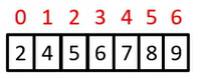
Iterative Binary Search in Code
- iterative_binary_search.py
- # Iterative Binary Search Function
- # It returns location of x in given array arr if present,
- # else returns -1
- def binarySearch(arr, l, r, x):
- while l <= r:
- mid = l + (r - l)/2;
- # Check if x is present at mid
- if arr[mid] == x:
- return mid
- # If x is greater, ignore left half
- elif arr[mid] < x:
- l = mid + 1
- # If x is smaller, ignore right half
- else:
- r = mid - 1
- # If we reach here, then the element was not present
- return -1
- # Test array
- arr = [ 2, 3, 4, 10, 40 ]
- x = 10
- # Function call
- result = binarySearch(arr, 0, len(arr)-1, x)
- if result != -1:
- print "Element is present at index %d" % result
- else:
- print "Element is not present in array"
Recursive Binary Search in Code
- recursive_binary_search.py
- # Python Program for recursive binary search.
- # Returns index of x in arr if present, else -1
- def binarySearch (arr, l, r, x):
- # Check base case
- if r >= l:
- mid = l + (r - l)/2
- # If element is present at the middle itself
- if arr[mid] == x:
- return mid
- # If element is smaller than mid, then it can only
- # be present in left subarray
- elif arr[mid] > x:
- return binarySearch(arr, l, mid-1, x)
- # Else the element can only be present in right subarray
- else:
- return binarySearch(arr, mid+1, r, x)
- else:
- # Element is not present in the array
- return -1
- # Test array
- arr = [ 2, 3, 4, 10, 40 ]
- x = 10
- # Function call
- result = binarySearch(arr, 0, len(arr)-1, x)
- if result != -1:
- print "Element is present at index %d" % result
- else:
- print "Element is not present in array"
Analysis of Binary Search
- In Binary Search, we choose an index that cuts the remaining portion of the array in half
- We repeat this until we either find the value we are looking for, or we reach a subarray of size 1
- If we start with an array of <m>size n</m>, we can cut it in half <m>log_2 n</m> times
- Hence, Binary Search has logarithmic <m>(log n)</m> time complexity in the worst and average cases, and constant time complexity in the best case
- For an array of size 1000, this is approx. 100 times faster than linear search (<m>2^10</m> ≈ 1000 when neglecting constant factors)
Conclusion
- Linear Search has linear time complexity
- Binary Search has logarithmic time complexity
- For large arrays, Binary Search is far more efficient than Linear Search
- However, Binary Search requires that the array is sorted
- If the array is sorted, Binary Search is
- Approx. 100 times faster for an array of size 1000 (neglecting constants)
- Approx. 50 000 times faster for an array of size 1 000 000 (neglecting constants)
- Significant improvements like these are what make studying and analysing algorithms worthwhile
Week 12: Benchmarking
Benchmarking Algorithms in Python
Overview
- Motivation for benchmarking
- Time in Python
- Benchmarking a single run
- Benchmarking multiple statistical runs
Motivation for Benchmarking
- Benchmarking or a posteriori analysis is an empirical method to compare the relative performance of algorithms implementations.
- Experimental (e.g running time) data may be used to validate theoretical or a priori analysis of algorithms
- Various hardware and software factors such system architecture, CPU design, choice of Operating System, background processes, energy saving and performance enhancing technologies etc. can effect running time.
- Therefore it is prudent to conduct multiple statistical runs using the same experimental setup, to ensure that your set of benchmarks are representative of the performance expected by an “average” user.
Time in Python
- Dates and times in Python are presented as the number of seconds that have elapsed since midnight on January 1st 1970 (the “unix epoch”)
- Each second since the Unix Epoch has a specific timestamp
- Can import the time module in Python to work with dates and times
- e.g start_time = time.time() # gets the current time in seconds
- e.g 15555001605 is Thursday, 11 April 2019 16:53:25 in GMT
Benchmarking a single run
import time

#log the start time in seconds
start_time = time.time()

#call the function you want to be benchmarked

#log the start time in seconds
end_time = time.time()

#calculate the elapsed time
time_elapsed = end_time - start_time
Benchmarking multiple statistical runs
import time

num_runs = 10 # number of times to test the function
results = [] # array to store the results for each test

# benchmark the function
for r in range(num_runs):
   # log the start time in seconds
   start_time = time.time()
   # call the function that you want to benchmark

   # log the end time in seconds
   end_time = time.time()

   # calculate the elapsed time
   time_elapsed = end_time - start_time

   results.append(time_elasped)
- benchmark.py
- from numpy.random import randint
- from time import time
- def Bubble_Sort(array):
- # your sort code
- sorted=array
- return sorted
- def Merge_Sort(array):
- # your sort code
- sorted=array
- return sorted
- def Counting_Sort(array):
- # your sort code
- sorted=array
- return sorted
- def Quick_Sort(array):
- # your sort code
- sorted=array
- return sorted
- def Timsort(array):
- # your sort code
- sorted=array
- return sorted
- # The actual names of your sort functions in your code somewhere, notice no quotes
- sort_functions_list = [Bubble_Sort, Merge_Sort, Counting_Sort, Quick_Sort, Timsort]
- # The prescribed array sizes to use in the benchmarking testst
- for ArraySize in (100, 250, 500, 750, 1000, 1250, 2500, 3750, 5000, 6250, 7500, 8750, 10000):
- # create a randowm array of values to use in the tests below
- testArray = randint(1,ArraySize*2,ArraySize)
- # iterate throug the list of sort functions to call in the test
- for sort_type in sort_functions_list:
- # and test every function ten times
- for i in range(10):
- start=time()
- sort_type(testArray)
- stop=time()
- print('{} {} {} {}'.format(sort_type, ArraySize, i, (stop-start)*1000))
Useful References
Python 3 time documentation: https://docs.python.org/3/library/time.html
Python Date and Time Overview https://www.tutorialspoint.com/python/python_date_time.htm
Discussions of benchmarking issues in Python (advanced material) https://www.peterbe.com/plog/how-to-do-performance-micro-benchmarks-in-python